Evolving Gaussian Mixture Models for Classiﬁcation

Simon Reichhuber

and Sven Tomforde

Intelligente Systeme, Christian-Albrechts-Universit

at zu Kiel, Kiel, Germany

Keywords:

Gaussian Mixture Models, Evolutionary Algorithms, Classiﬁcation, Human Activity Recognition.

Abstract:

The combination of Gaussian Mixture Models and the Expectation Maximisation algorithm is a powerful tool

for clustering tasks. Although there are extensions for the classiﬁcation task, the success of the approaches is

limited, in part because of instabilities in the initialisation method, as it requires a large number of statistical

tests. To circumvent this, we propose an ’evolutionary Gaussian Mixture Model’ for classiﬁcation, where a

statistical sample of models evolves to a stable solution. Experiments in the domain of Human Activity Recog-

nition are conducted to demonstrate the sensibility of the proposed technique and compare the performance to

SVM-based or LSTM-based approaches.

1 INTRODUCTION

In intelligent technical systems, e.g. referring to

concepts from the Autonomic (Kephart and Chess,

2003) or Organic Computing (M

uller-Schloer and

Tomforde, 2017) domains, decisions about appropri-

ate behaviour are typically taken based on a model

of the current perceptions. In many cases, this re-

quires continuous processing and classiﬁcation of

multi-dimensional sensor data. A large variety of

techniques can be found in literature that is applica-

ble to this task (D’Angelo et al., 2019) – but only a

few techniques can provide an estimate of the associ-

ated uncertainty in addition to the classiﬁcation deci-

sion. Classiﬁers based on Gaussian Mixture Models

(GMM) (Heck and Chou, 1994) have been shown to

come with a set of advantages including an inherent

estimate if uncertainty and a probability distribution

for the corresponding classes.

Consider human activity recognition (HAR)

(Kong and Fu, 2018) as an example for a classiﬁca-

tion task in intelligent systems. Here, the behaviour

of a human user is perceived by sensors, e.g. in terms

of gyroscope, accelerometer or magnetometer avail-

able on a smartphone. The incoming data stream of

the different sensors is pre-processed online, possi-

bly segmented into smaller parts, and classiﬁed. The

classiﬁcation can consider basic activities such as sit-

ting, walking, or running – but also more sophisti-

cated activities such as cycling or playing football.

https://orcid.org/0000-0001-8951-8962

https://orcid.org/0000-0002-5825-8915

Technically, these known activities are represented by

expected patterns and compared to the currently ob-

served patterns.

A standard approach for applying GMMs (or bet-

ter CMM: classiﬁers based on GMM) to HAR is

to run the Expectation Maximisation algorithm on

large sets of training data. In this paper, we pro-

pose an alternative approach: We aim at evolving the

CMM/GMM using evolutionary operators. Hence,

the contribution of the paper is twofold: It deﬁnes the

underlying evolutionary including the operators and

presents a detailed study on GMM-based HAR data

sets.

The remainder of this paper is organised as fol-

lows: Section 2 brieﬂy reviews the related literature of

GMMs, classiﬁcation, and Evolutionary Algorithms.

Next, we give a short recap of the used algorithms

(Section 3) which also leads to the used reference

baseline approach (Section 3.4). Then, in Section 4,

we present our methodology of evolving GMMs for

classiﬁcation. Subsequently, we explain the experi-

mental setup and present its results in Section 5. Fi-

nally, we give a short outlook to our further research

(Section 6) and summarise our ﬁndings in Section 7.

2 RELATED WORK

Gaussian Mixture Models (GMMs) has been fre-

quently used in the literature for the sake of a small-

dimensional representation. For example, in the

case of GMM-based adaptive knot placement for B-

964

Reichhuber, S. and Tomforde, S.

Evolving Gaussian Mixture Models for Classiﬁcation.

DOI: 10.5220/0010984900003116

In Proceedings of the 14th International Conference on Agents and Artiﬁcial Intelligence (ICAART 2022) - Volume 3, pages 964-974

ISBN: 978-989-758-547-0; ISSN: 2184-433X

Splines (Zhao et al., 2011), projection pursuit with

GMMs (Scrucca and Seraﬁni, 2019), or as features

for Support Vector Machines (in this context, the

representation is also called “Universal Background

Model” (You et al., 2010a)). Another ﬁeld that

uses the beneﬁts of GMMs is the Organic Comput-

ing (OC) domain. The robustness against sensor

noise and the advantage to analyse the knowledge

represented by a GMM are two important charac-

teristics making it attractive for constructors of such

self-adapative and self-aware systems (J

anicke et al.,

2016; M

uller-Schloer and Tomforde, 2017). Some

OC properties are guaranteed (with OC properties be-

ing a superset of self-* properties as originally deﬁned

for Autonomic Computing in (Kephart and Chess,

2003)), for instance adding new sensors to observa-

tion space (self-improving) and replacing defect ones

(self-healing). In decision-making problems, GMMs

are used for the detection of optimal actions which

was formulated as a classiﬁcation problem (M

uller-

Schloer and Tomforde, 2017). These GMM-based

classiﬁers are denoted as CMMs and have been used

in several applications throughout the last decades,

such as speaker identiﬁcation (del Alamo et al., 1996;

Ozerov et al., 2011; Qi and Wang, 2011), language

recognition (You et al., 2010b), Arabic sign language

recognition (Deriche et al., 2019), face video veriﬁ-

cation (Li and Narayanan, 2011), limb motion classi-

ﬁcation using continuous myoelectric signals (Huang

et al., 2005), or classiﬁcation of sequences observed

in electrocardiogram streams (Martis et al., 2009).

Due to the inherent robustness against noise and ex-

plicit modelling of the underlying uncertainties in

classiﬁcation tasks, GMMs have been shown to be a

powerful tool for human activity recognition (HAR)

anicke et al., 2016). In typical examples, the prin-

ciples of using accelerometer data from smartphones

(with a sampling rate of about 20 Hz to 40 Hz) for mo-

tion detection was shown in (Lau and David, 2010)

and recently has been reﬁned in (Garcia-Gonzalez

et al., 2020). Thus, we rely on HAR as a use case

in this article.

3 FOUNDATIONS OF GAUSSIAN

MIXTURE MODELS AND

EVOLUTIONARY

ALGORITHMS

This section brieﬂy summarises the technical basis of

our contribution. It, therefore, introduces the concept

of GMMs and explains how they can be turned into

classiﬁers.

3.1 GMM

A Gaussian Mixture Model (GMM) is the superpo-

sition of multiple (here J) Gaussians called compo-

nents (cf. Eq. (1)). Each component j has its own

set of parameters: the mean vector µ

which de-

scribes its location and a covariance matrix Σ

that

describes its shape. To ensure that the GMM rep-

resents a valid density (i.e.,

P(x)dx = 1) so-called

mixture coefﬁcients π

are introduced for each com-

ponent (cf. Eq. (2) and Eq. (3) for given constraints).

P(x

x) =

∑

j=1

· N (x

x|µ

,Σ

) (1)

0 ≤π

≤ 1 (2)

1 =

∑

j=1

(3)

, j

N (x

|µ

,Σ

)

P(x

)

(4)

The probabilities γ

, j

(cf. Eq. (4)) are called respon-

sibilities and indicate to what degree a given sample

belongs to a component j.

The parameters for a GMM can be ﬁtted using

standard Expectation-Maximisation (EM), or varia-

tional inference (Bishop, 2006) on a suitable train-

ing set X

train

. An implementation for variational

Bayesian inference for GMM can be found, e.g., in

(Gruhl et al., 2021). Belonging to the class of gen-

erative probabilistic models, a GMM can be used to

sample from it. That is, to generate distinct data sets

that have the same statistical properties as the used

training data. The sampling process is twofold. The

ﬁrst step is to draw

j from a categorical distribution

(also called multinoulli) described by the mixture co-

efﬁcients π

(cf. Eq. (5)). In the second step,

j indi-

cates from which of the Gaussian components a sam-

ple is drawn (cf. Eq. (6)). By repeating this procedure

we can sample a whole data set X

∗

with the same sta-

tistical properties as the training set X

train

j ' Cat(π

,...,π

) (5)

∗

' N (µ

,Σ

) (6)

3.2 CMM

Although GMMs are popular for clustering (McLach-

lan and Rathnayake, 2014; Chen et al., 2020), they

have also been extended for classiﬁcation. For exam-

ple, in (M

uller-Schloer and Tomforde, 2017), classi-

ﬁer based on Gaussian Mixture Models are denoted

as CMMs.

Evolving Gaussian Mixture Models for Classiﬁcation

965

Similar as in (M

uller-Schloer and Tomforde,

2017), we deﬁne the classiﬁcation model with

GMMs, starting with the class conclusions p(c| j), for

each component j:

p(c| j) = ξ

j,c

∑

x∈X

x, j

, (7)

Where X

are the samples in X assigned with label

c and N

∑

i=1

, j

is the sum of the responsibilities

of component j.

Then, the class posterior is given by:

p(c|x

x) =

∑

j=1

p(c| j) · p( j|x

x) =

∑

j=1

j,c

· γ

x, j

, (8)

Finally, the discrimination function is constructed

by calculating the a-posterior of the class probabili-

ties:

h(x

) = arg max



p(c|x



(9)

The ﬁnal classiﬁcation procedure using CMMs

consist of four steps:

(1) Initialisation

(2) K-Means reﬁnement

(3) EM-Updates

(4) Evaluation

The ﬁrst step, (1) Initialisation, shall provide initial

values for the means µ

and the covariance matrix Σ

of each component j in the CMM. This can either be

randomly done (cf. Reference baseline in Section 3.4)

or with an advanced procedure (cf. Evolved CMMS

in Section 4). To guarantee that Σ

is positive deﬁnite,

we can use the steps in Eq. (10), Eq.(11), and Eq.(12)

to generate random positive deﬁnite matrices:

M := (m

i, j

)

1≤i, j≤n

where m

i, j

∼ U

[−1,1]

(10)

M ← 0.5 · (M + M

) (11)

M ← M + n · 11

(12)

Subsequently, it is reasonable to stabilise the

means and distribute them according to the density

of the input space by applying a K-Means procedure

resulting in step (2) K-Means reﬁnement. Since K-

Means does not refer to labels, some more complex

classes are modelled by more components than other

classes. Afterwards, we apply EM-updates in step

(3) EM-Updates until a predeﬁned stop criterion is

reached. The latter can either be a total number of

iterations, or a certain threshold denoting the change

in the likelihood of drawing X from the current CMM

to the one of the last EM-Update ∆P(X |π

π,µ

µ,Σ

Σ). In

the end, we evaluate in step (4) Evaluation the dif-

ferences between the CMM model predictions of an

unseen test set ˆy

test

and the provided labels of this test

set y

test

. Finally, the measured classiﬁcation error is

deﬁned as our classiﬁcation performance.

3.3 Evolutionary Algorithms

Evolutionary Algorithms (EAs) are a powerful tool

for multi-dimensional minimisation/maximisation

problems. Given an input space X and a multi-

dimensional function f : X

− > R the goal is to

ﬁnd an input x

∗

maximising the function f , i.e.

∗

= argmax

x∈X

f (x). One of the pioneers of the

idea of evolving some randomly found solutions

by means of evolutionary operators (i.e. selection,

recombination, and mutation) was John H. Holland

who deﬁned one of the ﬁrst Genetic Algorithms in

the year 1975(Holland, 1975). Given a set of N

uniformly-distributed individuals, denoted as popula-

tion P , as seen in Algorithm 1 in each iteration the

individuals’ ﬁtness is calculated (CalculateFitness()),

based on the ﬁtness value, the most powerful indi-

viduals are selected (Selection()) for a recombination

procedure (Recombination()). In the end, random

mutation is applied to all of the novel individuals

Mutation() which form the next generation. Hence,

these iterations are also called generations g. The

algorithm terminates either after a previously-deﬁned

maximum number of generations g < G, or the

best-found ﬁtness value is above a certain threshold

τ ∈ R .

Algorithm 1: The canonical GA algorithm.

1: function GA(X, f )

2: P

(0)

← Initialisation()

3: g ← 0

4: while bestFitness(P

(g)

) < τ AND g < G do

5: Fitness ← CalculateFitness( f , P

(g)

)

6: Parents ← Selection(P

(g)

)

7: Offspring ← Recombination(Parents)

8: P

(g+1)

← Mutation(Offspring)

9: g ← g + 1

10: end while

11: return x

∗

, f (x

∗

), g

12: end function

3.4 Reference Baseline

As a reference baseline, we initialise a population

of CMMs by means of uniform-randomly distributed

conﬁgurations of the parameters: responsibilities

, j

, means µ

, and covariance matrices Σ

The com-

mon way to ﬁnd the most suitable CMM represen-

tation with f (X|Ω) ∼ Y is to uniformly initiate the

model parameters multiple times, and ﬁnd the centres

ICAART 2022 - 14th International Conference on Agents and Artiﬁcial Intelligence

966

of classes via K-Means iterations. Afterwards, the

EM-Algorithm is applied and the best initialisation in

terms of classiﬁcation error is kept. Given the number

of generations G and the population size N

, the evo-

lution of CMMs requires GN

evaluations. With the

same number resulting in similar computing time, one

can compare the evolutionary setting with the random

initialisation and subsequent K-Means.

4 METHODOLOGY

4.1 Evolution of CMMs

By the term ”Evolved Machine Learning” we mean

the maximisation of the performance of a machine

learning model through evolutionary algorithms. In

this process, a population is created that consists of

machine learning models with randomly selected hy-

perparameter conﬁgurations.

max

θ∈Θ

π(θ) (13)

Encoding

In the case of CMMs we deﬁne individual i of the

population as:

[i]



[i]

,µ

[i]

,Σ

[i]



(14)

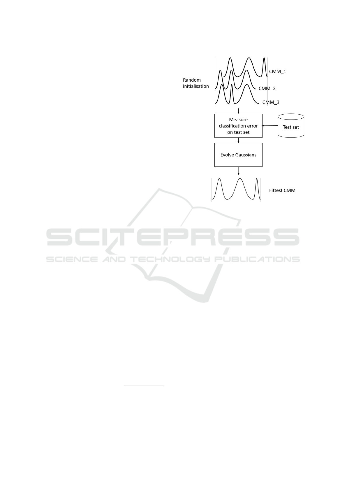
Fitness Function

Furthermore, the ﬁtness function is given by the clas-

siﬁcation performance that we are interested in. That

means, for each ﬁtness call we have to follow the

whole classiﬁcation procedure as we deﬁned in Sec-

tion 3.2. Based on this ﬁtness value, we are able to ap-

ply Evolutionary Algorithms and ﬁlter out the ﬁttest

individual after a maximum number of N

genera-

tions has been evolved (cf. Figure 1. Since we are

dealing with highly unbalanced datasets with |{y ∈

Y |y = c

}| << |{y ∈ Y |y = c

}| for some classes

∈ C , we decided to mostly concern the balanced

accuracy in our experiments. Given a set of true labels

Y := {y}

i=1

and model prediction

Y = { f (x

)}

i=1

{ ˆy

}

i=1

, the balanced accuracy weights each accuracy

is deﬁned as in (Velez et al., 2007) (cf. Eq. 15).

balanced-accuracy(Y ,

Y ) =

∑

i=1

}

( ˆy

)

|{y

∈ Y |y

= y

(15)

where χ

(ω) =



1 if ω ∈ S

0 if ω /∈ S

(16)

Figure 1: Schema of the procedure for evolving CMMs.

Selection

The parent population is found with respect to the ﬁt-

ness values of the individuals. The na

ıve selection

strategy that takes the top k individuals into account

leads to a poor diversity of the next generations. The

latter is solved by stochastic selection strategies. For

our approach, we used the selection strategy remain-

der stochastic sampling (Holland, 1975; Goldberg

et al., 1990; Blanco et al., 2001) based on the relative

ﬁtness. Remainder stochastic sampling combines the

strength of stochastic selection were even the weak-

est individual has a chance to be selected, similarly as

stochastic universal sampling, with a guaranteed se-

lection of individuals with a relative ﬁtness above the

average relative ﬁtness which limits the diversity but

stabilises the best solutions found so far.

Recombination

From the selection, there will be drawn two parents

and x

for pairing which results in two novel chil-

dren x

and x

. Since GMMs are probabilistic gen-

erative models, the simplest way to generate a new

child from two GMM parents would be to linearly

combine both parents and draw a new GMM from

the linear combination, which is also a GMM. Here

In order to keep track of the class imbalance also dur-

ing recombination. The ratio of the components per

class should remain. Therefore, we ﬁrst identify the

Evolving Gaussian Mixture Models for Classiﬁcation

967

components of a parent that is most likely generating

class c. Given a class c ∈ C , the class components of

parent p are deﬁned as:

∈N(J)

p(c

| j

) = j} (17)

Using the class components in Eq. 17, Parent 1 in-

duces her knowledge about the class complexity of

class c which can be estimated from the magnitude

of the class components |ι

(c)| to child 1, and par-

ent 2 analogous to child 2. This number is used

to determine the number of draws from the com-

bined component indices of parent 1 and parent 2,

i.e. ι

(c), representing the knowledge about

class c. Since

∑

|ι

(c)| = J, an iteration over

all classes sufﬁciently deﬁnes two new J-component

CMM children.

Mutation

Since each of the three CMM parameters π

[i]

, µ

[i]

and Σ

[i]

have different effects on the CMM, the

mutation should also be divided into three types.

Hence, there is the need for three mutation proba-

bilities: (1) a mixture-coefﬁcient mutation probabil-

ity p

, (2) a mean-mutation probability p

, and (3)

a correlation-matrix mutation probability p

. For the

mean-mutation, we simply implemented a uniformly

drawn one-step mutation. Because only a single di-

mension in a mean vector of the component of a

CMM is altered, the probability p

has to be ade-

quately small. The correlation-matrix mutation is ap-

plied by replacing a randomly selected row or column

with index i of the correlation matrix with a randomly

drawn row or column with values in [−1,1] where

to the i-th entry is added the number J. The addi-

tion keeps the positive deﬁniteness. Once an individ-

ual was chosen for mixture coefﬁcient mutation, we

apply a pairwise mixture coefﬁcient exchange of the

components i and j of an individual as in Eq. 18

s ← U[−s,s] , where s :=

(18)

← s (19)

← −s (20)

Elitism

Only, a small amount of the best individuals in the

population, denoted as elites, are immune to the mu-

tation operation and are added directly to the next

generation. Therefore, the parameter r

elite

deﬁnes the

fraction of elites in the population.

Algorithm 2: Evolved-CMMs as a combination of an EA

and CMMs. The negative loss function −L is set to the

balanced accuracy.

1: function EVOLVED-CMMS(X

train

, y

train

, X

test

)

2: X

train

← Z-norm(X

train

,µ

train

,σ

train

)

3: X

test

← Z-norm(X

test

,µ

train

,σ

train

)

4: Initialise population of CMMs P

(0)

5: while g < G do

6: for each i ∈ N(N

) do

7: CMM

[ﬁtness] ←

−L(y

test

,CMM

test

))

8: end for

9: Parents ←

RemainderStochasticalSampling

({CMM

}

i=1

10: Offspring ←

Recombination(Parents)

11: NextGeneration ←

Mutation(Parents ∪ Offspring) ∪ Elite

12: g ← g + 1

13: P

(g)

← NextGeneration

14: end while

15: CMM

∗

←

argmax

CMM∈CMM

(g)

−L(y

test

,CMM

test

))

16: score ← −L(y

test

,CMM

∗

test

))

17: return CMM

∗

,score

18: end function

4.2 Evolving Time-consuming Machine

Learning Models

One question is how to reduce the huge amount of

ﬂoating-point operations (FLOPs). Besides the in-

dividuals that are marked as elitists, there is also a

percentage of selected parents that are included un-

touched in the next generation. Since their model pa-

rameters already have been evaluated once, it makes

sense to keep track of unchanged individuals and pre-

vent a time-consuming re-computation of the ﬁtness.

Another runtime optimisation can be found in paral-

lelisation of the individuals of one generation within

the GPU as explained in (Chen et al., 2020).

5 EXPERIMENTS

In this section, we explain the conducted experi-

ments in the domain of HAR. The dataset was taken

from the contribution of Garcia-Gonzalez et. al

(Garcia-Gonzalez et al., 2020) and contains sensor

records from 19 smartphone-users who wear their

smart phone in daily-life and annotated their state of

activity by giving labels, i.e. inactive, active, walking,

ICAART 2022 - 14th International Conference on Agents and Artiﬁcial Intelligence

968

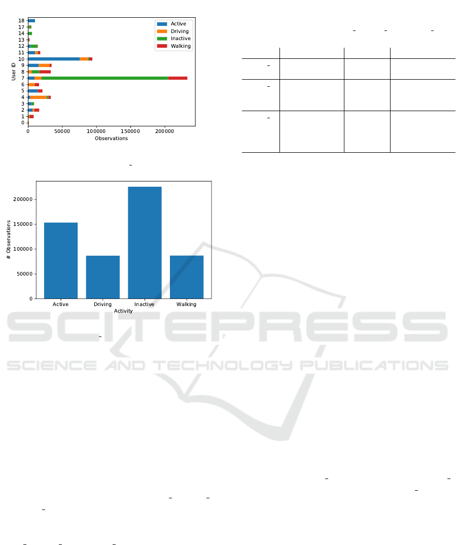
Figure 2: Total number of samples provided for each activ-

ity of each user in the dataset HAR 1.

Figure 3: Total number of samples provided for each of the

classes in the dataset HAR 1.

and driving. They sampled the streams with a sliding

window approach into 20 sec-chunks with an overlap

of 19 sec. In Figure 2, the distribution of the samples

per user is visualised.

Another characteristic of this dataset is the class

imbalance, which can be seen in Figure 3. These im-

balance should be taken into account by the classi-

ﬁcation and underlines the necessity of the balanced

accuracy, i.e. a na

ıve classiﬁer always predicting the

activity inactive would reach a accuracy of 43 %.

For the analysis of the optimal sensors, the au-

thors provided three different sets based on differ-

ent sensors, which we abbreviate HAR 1, HAR 2,

and HAR 3 in the remainder. The detailed sensor

equipment of each dataset can be seen in Table 1.

The differencies in the number of samples between

HAR 1, HAR 2, and HAR 3 is due to different user

equipment. The claimed objective of the authors of

(Garcia-Gonzalez et al., 2020) is to provide a dataset

from which machine learning algorithms can create a

orientation-independent, placement-independent, and

subject-independent predictor for the activity. Even if

further experiments are needed to afﬁrm the claim for

more than the included 19 subjects, more placements,

and more orientations (which were not been deﬁned,

Table 1: Sensor equipment, support, and involved users of

each of the three datasets HAR 1, HAR 2, and HAR 3 pro-

vided by (Garcia-Gonzalez et al., 2020).

Name Used sensors #samples User IDs

HAR 1 Accelerometer

GPS

182387 All users

(ID 0 to ID 18)

HAR 2 Accelerometer

Magnetometer

GPS

177246 Missing IDs:

14, 15, 16, 18

HAR 3 Accelerometer

Gyroscope

Magnetometer

GPS

164762 Missing Ids:

4, 14-18

hence, determined by the individual behaviour of the

users), the large variety of these attributes induces a

high noise in the dataset. In contrast to this noise

which is not well understood, for the reduction of the

pure sensor noise, there are simple methods available

in machine learning. For this reason, the author pro-

vide a preprocessing with low-pass ﬁlter and suggest

to extract the following statistical features for each

sensor:

• Mean

• Minimum

• Maximum

• Variance

• Mean absolute deviation

• Interquartile range

Counting the number of extracted values per sensor

per timestamp, there are three for the accelerometer,

three for the gyroscope, and three for the magnetome-

ter. Additionally, for the GPS, there can be extracted

six values: latitude, longitude, altitude, speed, bear-

ing, and accuracy.

Given three values measured by the accelerome-

ter, six values extracted from the GPS, and for each

six statistical features, it sums up to 6 · (3 + 6) = 54

features for the HAR 1 dataset, analogous for HAR 2

6 · (3 + 3 + 6) = 72 features, and for HAR 3 6 · (3 +

3 + 3 + 6) = 90 features. Using these features, the ﬁt-

ness function requires a training phase of a CMM on

67 % of the dataset with the following parameters in

Table 2 and a test phase calculating the balanced ac-

curacy on 33 % of the dataset. Before the training or

testing, the samples were z-normalised based on vari-

ance and mean found in the training set.

With this CMM setting, we initialised the evolu-

tionary algorithm with the parameters in Table 3. Be-

cause of the limtited computing time, the parameters

were manually optimised. Further improvements in

the efﬁciency of the algorithm may allow a compre-

hensive hyperparameter tuning.

Evolving Gaussian Mixture Models for Classiﬁcation

969

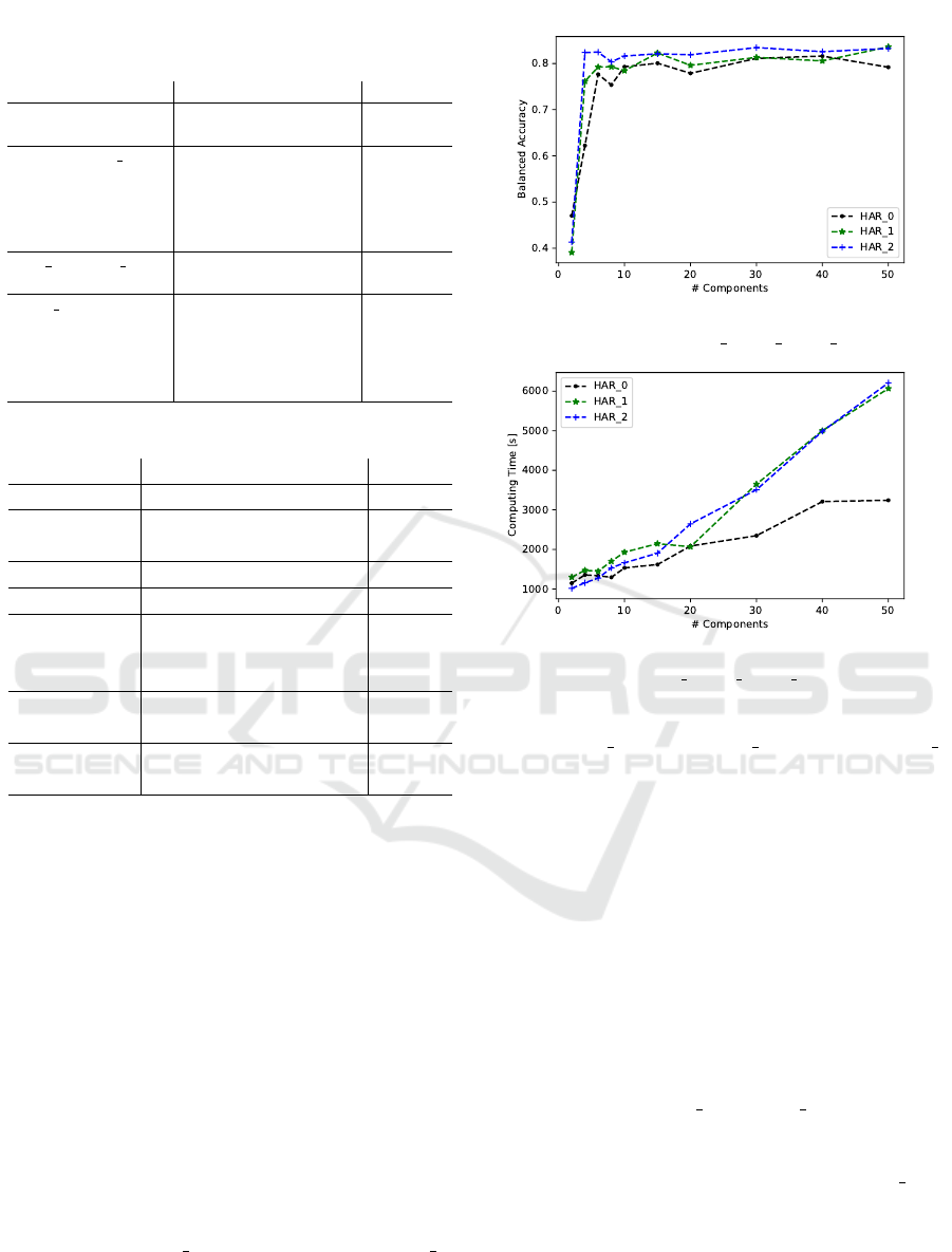
Table 2: Parameters used for training CMMs without evo-

lutionary adaptation.

Parameter Description Value

J Number of Gaussian

components

covariance type Characteristics of the

positive deﬁnite co-

variance matrix (e.g.

full, diagonal, con-

stant)

full

em updates max Maximum number of

EM updates

100

em tolerance Stop criterion for EM

updates if the change

of the likelihood

∆P(X|π

π,µ

µ,Σ

Σ) is

below this threshold

1 × 10

−3

Table 3: Parameters used for the evolutionary algorithm.

Parameter Description Value

Population size 100

Number of genera-

tions

100

Parents ratio 50 %

Elites ratio 1 %

Mutation proba-

bility for mixture-

coefﬁcient

1 %

Mutation probability

for means

1 %

Mutation probability

for covariance matrix

1 %

Time Complexity versus Performance Trade-off

The setting of the parameters in Table 2 comes with

a trade-off decision between accuracy (cf. Figure 4)

and computing time (cf. Figure 5). Therefore, we

analysed the balanced accuracy of models of varying

complexity. The higher the number of components

in a single CMM, the larger is its model complexity.

As a drawback, this model has to be called for each

ﬁtness call.

Therefore, a good trade-off between the perfor-

mance reaching a level of 81.108% balanced accuracy

and limiting the computing time to 2347 sec (for com-

parison, using 40 components the computing time in-

creases to 3209 sec) are 30 components. It is note-

worthy that also the number of features inﬂuences the

computing time and there is a break point between

54 features of HAR 1 and 72 features of HAR 2,

whereas the balanced accuracy is quit high for all

datasets.

In comparison to the authors of the dataset who

applied support vector machines for the classiﬁca-

Figure 4: Balanced accuracy of evolved GCC trained on

each of the data sets, i.e. HAR 0, HAR 1, HAR 2.

Figure 5: Computing time of evolved GCC trained on each

of the data sets, i.e. HAR 0, HAR 1, HAR 2.

tion (Garcia-Gonzalez et al., 2020) with a mean accu-

racy of HAR 1 67.53 %, HAR 2 74.39 %, and HAR 3

69.28 %, the evolved CMMs predict up to a balanced

accuracy of 80.03 % (cf. Figure 4). The baseline

(see Section 4) eventually reached a maximum bal-

anced accuracy of 79.324 %. But on average it only

got 75.916 % with a standard deviation of 1.464 %.

With this, the baseline is in the near of the evolu-

tionary algorithm but the chances of having an ap-

propriate CMM initialisation are in general not suf-

ﬁcient for a secure guarantee. In contrast to the ran-

dom initialisation, because of elitism in the evolving

CMMs, the ﬁtness value history is monotonically in-

creasing. Therefore, in all of the runs, the evolved

CMMs reached a stable solution above 80 % balanced

accuracy as seen in Figure 6. We also assume that the

larger sensor sets HAR 2 and HAR 3 would increase

further with more generations and more computing

time. With respect to the computing time and the best

results, we would decide to use dataset HAR 1 for

HAR classiﬁcation with Gaussians and statistical fea-

tures.

ICAART 2022 - 14th International Conference on Agents and Artiﬁcial Intelligence

970

Table 4: Classiﬁcation results of evolved CMMs tested on

33 % of the samples in the datasets HAR 1, HAR 2, and

HAR 3.

precision recall f1-score support

Active 0.85 0.58 0.69 50741

Driving 0.87 0.83 0.85 28768

Inactive 0.79 0.93 0.86 74398

Walking 0.66 0.76 0.70 28480

accuracy 0.79 0.79 0.79 1.0

macro avg 0.79 0.78 0.78 182387

weighted avg 0.80 0.79 0.79 182387

(a) Classiﬁcation results of evolved CMMs tested on 182k

samples of HAR dataset with features based on triaxial ac-

celerometer sensor and GPS.

precision recall f1-score support

Active 0.79 0.62 0.70 47107

Driving 0.73 0.92 0.81 28613

Inactive 0.80 0.95 0.87 72676

Walking 0.90 0.57 0.70 28850

accuracy 0.79 0.79 0.79 1.0

macro avg 0.80 0.77 0.77 177246

weighted avg 0.80 0.79 0.79 177246

(b) Classiﬁcation results of evolved CMMs tested on 177k

samples of HAR dataset with features based on triaxial ac-

celerometer, triaxial gyroscope, and GPS.

precision recall f1-score support

Active 0.72 0.66 0.69 46386

Driving 0.91 0.75 0.82 20332

Inactive 0.81 0.91 0.85 70456

Walking 0.75 0.69 0.72 27588

accuracy 0.78 0.78 0.78 1.0

macro avg 0.79 0.75 0.77 164762

weighted avg 0.78 0.78 0.78 164762

samples of HAR dataset with features based on triaxial ac-

celerometer, triaxial gyroscope, GPS, and magnetometer.

6 FURTHER RESEARCH

The presented approach offers a potential interface

to adapt the evolution principles towards control of

diversity using, e.g., self-betting or external-betting

mechanisms as proposed in (Reichhuber and Tom-

forde, 2021). There are two options to enrich the

algorithm with betting capabilities. Either each in-

dividual is given the possibility to bet on itself (self-

betting Evolutionary Algorithm), or we introduce an-

other bet population which is evolved simultaneously

to the GCCs and its only objective is to learn how to

bet on the individuals of the current population.

(a) Best ﬁtness value history of evolved CMMs tested

on 182k samples of HAR dataset with features based on

triaxial-accelerometer sensor and GPS.

(b) Best ﬁtness value history of evolved CMMs tested on

177k samples of HAR dataset with features based on triaxial

accelerometer, triaxial gyroscope, and GPS.

164k samples of HAR dataset with features based on triaxial

accelerometer, triaxial gyroscope, GPS, and magnetometer.

Figure 6: Fitness value history over 100 generations of

evolving CMMs tested on the datasets HAR 1, HAR 2, and

HAR 3.

Evolving Gaussian Mixture Models for Classiﬁcation

971

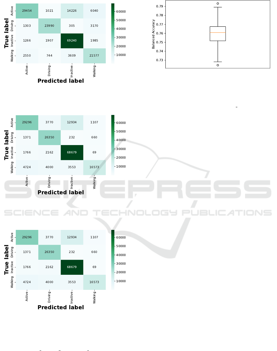
(a) Confusion matrix of evolved CMMs tested on 182k

samples of HAR dataset with features based on triaxial-

accelerometer sensor and GPS.

(b) Confusion matrix of evolved CMMs tested on 177k

samples of HAR dataset with features based on triaxial ac-

celerometer, triaxial gyroscope, and GPS.

ples of HAR dataset with features based on triaxial ac-

celerometer, triaxial gyroscope, GPS, and magnetometer.

Figure 7: Confusion matrices of evolving CMMs tested on

the datasets HAR 1, HAR 2, and HAR 3.

Figure 8: Boxplot diagram with the 25th and the 75th per-

centile of the balanced accuracy distribution found with the

baseline reference. In 100000 iterations the best-found ini-

tialisations of GCCs resulted in a maximum balanced accu-

racy of 79.324 % and a median (orange line) of 76.083 %.

The tests were driven on the data set HAR 0.

Since the latter would increase the time complex-

ity of the algorithm, a solution for reducing the time

complexity of evolving GCCs is required. Due to the

matrix inversion, the time complexity of training a

single CMM with n samples of dimensions d in k it-

erations of EM updates is O(nkd

). Since the latter is

required for each ﬁtness update of the individuals in

a population, there are two more factors: (i) the num-

ber of generations g and (ii) the population size N that

needs to be considered. In total, the time complexity

for the evolved GCC algorithm is O(gN(nkd

)).

However, for the experiments, we were able to

limit the actual costs to an affordable amount of com-

puting time. That is, we limited the number of EM

iterations to a maximum of 100 and also used a min-

imum update delta of 1e − 3 as stop criterion, which

reduces the actual duration to a spendable amount of

computing time.

Regarding the high time complexity, a further im-

provement of the evolved CMM algorithm would be

a replacement of the EM updates with a low-cost ap-

proximation. Using fast Incremental Gaussian Mix-

ture Models, as presented in (Pinto and Engel, 2015),

and limiting the stream size s for each individual in

the population, the time complexity of the algorithm

can be reduced to O(gN(skd

)). However, the in-

creasing performance lost needs to be evaluated in

further experiments.

For general improvements of the HAR predic-

tion, there might be taken more features into account.

These might be adapted in an automated feature se-

lection procedure tailored for a speciﬁc set of HAR

activities. A good starting point for this, can be found

in the library Time Series Feature Extraction Library

(TSFEL) (Barandas et al., 2020) where the authors

provide a list of general purpose time series features.

For further improvements to the prediction perfor-

mance, the datasets might be uniformed to a bench-

ICAART 2022 - 14th International Conference on Agents and Artiﬁcial Intelligence

972

mark set including other daily life activities, like in

(Leutheuser et al., 2013).

7 SUMMARY

This article presented a novel approach of evolving

Gaussian Mixture Models (GMMs) that are applied to

classiﬁcation tasks, therefore called Classiﬁer based

on GMM (CMM). We explained that GMM and their

particular variant of CMM are powerful tools that

have been shown to obtain very good results in many

domains and data sets. The current state of the art in

training them lies in the usage of k-means and expec-

tation maximisation, resulting in the most appropri-

ate shape of the Gaussians. However, this is charac-

terised by strong efforts in the training procedure. In

contrast, our approach aims at utilising the principles

of evolutionary computation. Hence, we presented

our methodology in detail, including the encoding

scheme, the deﬁnition of two novel genetic opera-

tors (i.e. mutation and recombination), and the result-

ing steps of the evolutionary process. Furthermore, a

baseline reference of random K-Means initialisation

is presented. In an experimental section, we demon-

strated the potential beneﬁt of evolved GMMs/CMMs

using human activity recognition (HAR) as challeng-

ing use case. In considering various data sets of HAR,

we analysed the capability of evolved CMMs to pre-

dict the correct activities. In total, a balanced accu-

racy of above 80 % has been achieved, which is par-

ticularly comparable to other approaches of the state-

of-the-art while simultaneously allowing for novel ad-

vantages from the evolutionary process.

REFERENCES

Barandas, M., Folgado, D., Fernandes, L., Santos, S.,

Abreu, M., Bota, P., Liu, H., Schultz, T., and Gam-

boa, H. (2020). Tsfel: Time series feature extraction

library. SoftwareX, 11:100456.

Bishop, C. M. (2006). Pattern Recognition and Ma-

chine Learning (Information Science and Statistics).

Springer-Verlag.

Blanco, A., Delgado, M., and Pegalajar, M. C. (2001).

A real-coded genetic algorithm for training recurrent

neural networks. Neural networks, 14(1):93–105.

Chen, C., Wang, C., Hou, J., Qi, M., Dai, J., Zhang, Y.,

and Zhang, P. (2020). Improving accuracy of evolving

gmm under gpgpu-friendly block-evolutionary pat-

tern. International Journal of Pattern Recognition and

Artiﬁcial Intelligence, 34(03):2050006.

D’Angelo, M., Gerasimou, S., Ghahremani, S., Grohmann,

J., Nunes, I., Pournaras, E., and Tomforde, S. (2019).

On learning in collective self-adaptive systems: state

of practice and a 3d framework. In Proc. of 14th Int.

Symp. on Software Engineering for Adaptive and Self-

Managing Systems, pages 13–24.

del Alamo, C. M., Gil, F. C., Gomez, L. H., et al. (1996).

Discriminative training of gmm for speaker identiﬁ-

cation. In 1996 IEEE International Conference on

Acoustics, Speech, and Signal Processing Conference

Proceedings, volume 1, pages 89–92. IEEE.

Deriche, M., Aliyu, S. O., and Mohandes, M. (2019). An

intelligent arabic sign language recognition system

using a pair of lmcs with gmm based classiﬁcation.

IEEE Sensors Journal, 19(18):8067–8078.

Garcia-Gonzalez, D., Rivero, D., Fernandez-Blanco, E.,

and Luaces, M. R. (2020). A public domain dataset

for real-life human activity recognition using smart-

phone sensors. Sensors, 20(8):2200.

Goldberg, D. E. et al. (1990). Real-coded genetic algo-

rithms, virtual alphabets and blocking. Citeseer.

Gruhl, C., Sick, B., and Tomforde, S. (2021). Novelty de-

tection in continuously changing environments. Fu-

ture Generation Computer Systems, 114:138–154.

Heck, L. P. and Chou, K. C. (1994). Gaussian mixture

model classiﬁers for machine monitoring. In Proceed-

ings of ICASSP’94. IEEE International Conference on

Acoustics, Speech and Signal Processing, volume 6,

pages VI–133. IEEE.

Holland, J. (1975). Adaptation in natural and artiﬁcial sys-

tems, univ. of mich. press. Ann Arbor.

Huang, Y., Englehart, K., Hudgins, B., and Chan, A. (2005).

A gaussian mixture model based classiﬁcation scheme

for myoelectric control of powered upper limb pros-

theses. IEEE Transactions on Biomedical Engineer-

ing, 52(11):1801–1811.

anicke, M., Tomforde, S., and Sick, B. (2016). Towards

self-improving activity recognition systems based on

probabilistic, generative models. In 2016 IEEE

International Conference on Autonomic Computing

(ICAC), pages 285–291. IEEE.

Kephart, J. and Chess, D. (2003). The Vision of Autonomic

Computing. IEEE Computer, 36(1):41–50.

Kong, Y. and Fu, Y. (2018). Human action recog-

nition and prediction: A survey. arXiv preprint

arXiv:1806.11230.

Lau, S. L. and David, K. (2010). Movement recognition us-

ing the accelerometer in smartphones. In 2010 Future

Network & Mobile Summit, pages 1–9. IEEE.

Leutheuser, H., Schuldhaus, D., and Eskoﬁer, B. M. (2013).

Hierarchical, multi-sensor based classiﬁcation of daily

life activities: comparison with state-of-the-art al-

gorithms using a benchmark dataset. PloS one,

8(10):e75196.

Li, M. and Narayanan, S. (2011). Robust talking face video

veriﬁcation using joint factor analysis and sparse rep-

resentation on gmm mean shifted supervectors. In

2011 IEEE International Conference on Acoustics,

Speech and Signal Processing (ICASSP), pages 1481–

1484. IEEE.

Martis, R. J., Chakraborty, C., and Ray, A. K. (2009). A

two-stage mechanism for registration and classiﬁca-

Evolving Gaussian Mixture Models for Classiﬁcation

973

tion of ecg using gaussian mixture model. Pattern

Recognition, 42(11):2979–2988.

McLachlan, G. J. and Rathnayake, S. (2014). On the num-

ber of components in a gaussian mixture model. Wiley

Interdisciplinary Reviews: Data Mining and Knowl-

edge Discovery, 4(5):341–355.

uller-Schloer, C. and Tomforde, S. (2017). Organic

Computing-Technical Systems for Survival in the Real

World. Springer.

Ozerov, A., Lagrange, M., and Vincent, E. (2011). Gmm-

based classiﬁcation from noisy features. In Interna-

tional Workshop on Machine Listening in Multisource

Environments (CHiME 2011).

Pinto, R. C. and Engel, P. M. (2015). A fast incremental

gaussian mixture model. PloS one, 10(10):e0139931.

Qi, P. and Wang, L. (2011). Experiments of gmm based

speaker identiﬁcation. In 2011 8th International Con-

ference on Ubiquitous Robots and Ambient Intelli-

gence (URAI), pages 26–31. IEEE.

Reichhuber, S. and Tomforde, S. (2021). Bet-based evolu-

tionary algorithms: Self-improving dynamics in off-

spring generation. In ICAART (2), pages 1192–1199.

Scrucca, L. and Seraﬁni, A. (2019). Projection pursuit

based on gaussian mixtures and evolutionary algo-

rithms. Journal of Computational and Graphical

Statistics, 28(4):847–860.

Velez, D. R., White, B. C., Motsinger, A. A., Bush, W. S.,

Ritchie, M. D., Williams, S. M., and Moore, J. H.

(2007). A balanced accuracy function for epistasis

modeling in imbalanced datasets using multifactor di-

mensionality reduction. Genetic Epidemiology: the

Ofﬁcial Publication of the International Genetic Epi-

demiology Society, 31(4):306–315.

You, C. H., Lee, K. A., and Li, H. (2010a). Gmm-svm ker-

nel with a bhattacharyya-based distance for speaker

recognition. IEEE Transactions on Audio, Speech,

and Language Processing, 18(6):1300–1312.

You, C. H., Li, H., and Lee, K. A. (2010b). A gmm-

supervector approach to language recognition with

adaptive relevance factor. In 2010 18th European Sig-

nal Processing Conference, pages 1993–1997. IEEE.

Zhao, X., Zhang, C., Yang, B., and Li, P. (2011). Adaptive

knot placement using a gmm-based continuous opti-

mization algorithm in b-spline curve approximation.

Computer-Aided Design, 43(6):598–604.

ICAART 2022 - 14th International Conference on Agents and Artiﬁcial Intelligence

974