Metaheuristics-based Exploration Strategies

for Multi-Objective Reinforcement Learning

Florian Felten

1 a

, Gr

egoire Danoy

1,2 b

, El-Ghazali Talbi

3 c

and Pascal Bouvry

1,2 d

SnT, University of Luxembourg, Esch-sur-Alzette, Luxembourg

FSTM/DCS, University of Luxembourg, Esch-sur-Alzette, Luxembourg

University of Lille, CNRS/CRIStAL, Inria Lille, France

Keywords:

Reinforcement Learning, Multi-objective, Metaheuristics, Pareto Sets.

Abstract:

The ﬁelds of Reinforcement Learning (RL) and Optimization aim at ﬁnding an optimal solution to a problem,

characterized by an objective function. The exploration-exploitation dilemma (EED) is a well known subject

in those ﬁelds. Indeed, a consequent amount of literature has already been proposed on the subject and shown

it is a non-negligible topic to consider to achieve good performances. Yet, many problems in real life involve

the optimization of multiple objectives. Multi-Policy Multi-Objective Reinforcement Learning (MPMORL)

offers a way to learn various optimised behaviours for the agent in such problems. This work introduces a

modular framework for the learning phase of such algorithms, allowing to ease the study of the EED in Inner-

Loop MPMORL algorithms. We present three new exploration strategies inspired from the metaheuristics

domain. To assess the performance of our methods on various environments, we use a classical benchmark

- the Deep Sea Treasure (DST) - as well as propose a harder version of it. Our experiments show all of the

proposed strategies outperform the current state-of-the-art ε-greedy based methods on the studied benchmarks.

1 INTRODUCTION

Reinforcement Learning (RL) has recently drawn a

lot of interest after the recent successes of this tech-

nique when applied to various types of problems.

Early applications initially targeted game problems

Silver et al. (2016), while more and more real life

problems, e.g. protein structure prediction Jumper

et al. (2021), have lately been addressed.

Nonetheless, most of the RL literature consid-

ers single-objective problems where real world prob-

lems often deal with multiple, generally contradicting

objectives. For instance, an autonomous car could

have to ﬁnd a trade-off between battery usage and

the speed at which it reaches a destination. The class

of algorithms that aims at ﬁnding the best trade-offs

between these objectives using reinforcement learn-

ing is called Multi-Objective Reinforcement Learn-

ing (MORL). So far, little interest has been shown

in MORL compared to the amount of research being

https://orcid.org/0000-0002-2874-3645

https://orcid.org/0000-0001-9419-4210

https://orcid.org/0000-0003-4549-1010

https://orcid.org/0000-0001-9338-2834

held in RL.

The most frequent way of solving a multi-

objective problem with MORL is to reduce it to a

single-objective problem by merging the various ob-

jectives into a global one. The prominent merg-

ing function, called scalarization function, is a linear

weighted sum, but others exist e.g. Van Moffaert et al.

(2013). Despite its popularity, this approach has sev-

eral drawbacks. For example, ﬁnding the right scalar-

ization function is usually done via a trial and error

process, which is time consuming and can lead to sub-

optimal choices. Another example is that user prefer-

ences can be dynamically changing. In that case, the

algorithm would need to be entirely retrained for each

new user preference Hayes et al. (2021).

Multi-policy MORL algorithms address these is-

sues by learning multiple policies leading to good

trade-offs between objectives. These learning meth-

ods can be divided in two categories, outer-loop and

inner-loop Roijers et al. (2013); Hayes et al. (2021).

The outer-loop method, which is the most common,

consists in running multiple times single-objective RL

algorithms with varying parameters, as to aim for dif-

ferent trade-offs. The inner-loop method modiﬁes the

learning algorithm itself to simultaneously learn mul-

662

Felten, F., Danoy, G., Talbi, E. and Bouvry, P.

Metaheuristics-based Exploration Strategies for Multi-Objective Reinforcement Learning.

DOI: 10.5220/0010989100003116

In Proceedings of the 14th International Conference on Agents and Artiﬁcial Intelligence (ICAART 2022) - Volume 2, pages 662-673

ISBN: 978-989-758-547-0; ISSN: 2184-433X

tiple policies.

The exploration-exploitation dilemma (EED) con-

sists in ﬁnding a good trade-off between looking in

the neighborhood of known good solutions and ex-

ploring unknown regions. It can signiﬁcantly inﬂu-

ence the performance of RL algorithms. It has been

thoroughly studied in traditional RL settings Amin

et al. (2021) but rarely in multi-policy MORL. In fact,

to the best of our knowledge, no work has been ded-

icated to study the exploration question in inner-loop

algorithms yet Vamplew et al. (2017a).

This paper thus studies the EED for Multi-Policy

Inner-Loop MORL algorithms (MPILMORLs). It

presents three novel exploration strategies for MPIL-

MORLs inspired from the metaheuristic domain:

Pheromones-Based (PB), Count-Based (CB), Tabu-

Based (TB). These strategies are based on the idea

of repulsion from already visited state and actions.

In addition, a new episodic, deterministic bench-

mark environment, called Mirrored Deep Sea Trea-

sure (MDST) is introduced. This environment is a

harder version of the state-of-the-art Deep Sea Trea-

sure (DST) benchmark. Lastly, experiments are con-

ducted on the DST and MDST environments, show-

ing the three proposed strategies outperform state-of-

the-art techniques.

The remainder of this article is organized as fol-

lows: Section 2 describes related work, Section 3

presents a learning framework for multi-policy inner-

loop MORL algorithms as well as the three new ex-

ploration strategies, Section 4 contains our experi-

mental setup while results are presented and analysed

in Section 5. Finally Section 6 concludes our work

and provides some perspectives.

2 BACKGROUND

This section presents the related work and current

state-of-the-art upon which this paper builds. Sec-

tion 2.1 provides a short introduction to Reinforce-

ment Learning. Section 2.2 presents relevant work in

MORL. Finally, Section 2.3 introduces the EED in RL

and Optimization.

2.1 Reinforcement Learning

In reinforcement learning, an agent interacts with an

environment in order to maximize a reward signal.

The agent receives positive or negative feedback de-

pending on the actions it realized on the environment.

RL environments are usually modeled as Markov De-

cision Processes (MDP) Sutton and Barto (2018).

This paper restricts its study to deterministic

MDPs. A deterministic MDP is represented by a tu-

ple (S,A,r) where: S represents the set of possible

states the agent can observe in the environment, A is

the set of actions the agent can realize to interact with

the environment, r : S × A −→ R is the reward distri-

bution where r(s, a) represents the immediate reward

received after performing action a in state s.

The goal of single-objective RL algorithm is to

ﬁnd a policy π(a|s) which maps each state to a proba-

bility of taking action a in state s. An optimal policy,

denoted π

∗

, is one which maximizes its state-value

function:

(s) = E

∞

∑

k=0

r(s

t+k

) | s

= s

where E

[·] represents the expected value of a

variable given that the agent follows policy π, start-

ing from state s at time step t. γ ∈ [0,1] is a discount

factor, adjusting the importance of long term rewards.

Similarly, the value of taking action a in state s

under policy π, called action-value function of policy

π, is deﬁned as:

(s,a) = E

∞

∑

k=0

r(s

t+k

) | s

= s, a

= a

The main difference between RL and dynamic

programming (DP) is that the latter assumes a perfect

knowledge of the environment dynamics. Indeed, in

DP, the (S,A,r) tuple is known in advance and the al-

gorithm searches for the optimal policy whereas RL

does not know anything about the environment and

learns π

∗

by interacting with it. There exists a class of

RL algorithms which aim at learning a model of the

environment in order to be able to apply traditional

optimisation techniques, these are called model-based

RL Sutton and Barto (2018).

RL algorithms can learn on-policy, meaning the

agent follows the policy it is currently learning; or

off-policy, where the agent follows a behavioral pol-

icy which is different from the target policy being

learned.

2.2 Multi-Objective Reinforcement

Learning

The difference between traditional RL and MORL

is that the reward is a vector in the latter.

Thus, the rewards take a vector form r(s,a) =

(s,a), .. ., r

(s,a)), with m being the number of

objectives. These environments can be expressed

using Multi-Objective Markov Decision Processes

(MOMDPs).

Metaheuristics-based Exploration Strategies for Multi-Objective Reinforcement Learning

663

In that setting, the state-value function has a vector

form and is deﬁned as:

(s) = E

∞

∑

k=0

r(s

t+k

) | s

= s

The same reasoning applies to the action-value

function.

There exists two families of MORL algorithms

which aim at solving MOMDPs. The ﬁrst one learns

one policy based on a scalarization of the problem and

is referred to as single-policy algorithms. The second

one, called multi-policy algorithms, is the one consid-

ered in this work and detailed hereinafter.

2.2.1 Multi-Policy Reinforcement Learning

Algorithms

This family of MORL algorithms aim at learning mul-

tiple policies leading to various optimal points in the

objective space. This class of algorithms is generally

considered in scenarios similar to the one illustrated

in Figure 1. These algorithms are generally trained

off-line and executed online as the user preferences do

not need to be speciﬁed a priori Roijers et al. (2013);

Hayes et al. (2021). Because of this train-test per-

spective, the most important factor for quality mea-

surements of these algorithms is the quality of the ﬁ-

nal policies, rather than the rewards received during

learning Vamplew et al. (2011). In general, to ensure

optimality of the learned policies, the behavioral pol-

icy must guarantee to visit all the state-action pairs

in an inﬁnite horizon, as to sample the entire search

space Van Moffaert and Now

e (2014).

There are two ways to learn multiple policies

called outer-loop and inner-loop. The ﬁrst one re-

peats single-policy algorithms with different parame-

ters as to look for various policies e.g. Vamplew et al.

(2017a,b); Parisi et al. (2016); Oliveira et al. (2020).

MPILMORL. The second one, which is consid-

ered in this study, modiﬁes the learning algorithm it-

self to simultaneously learn multiple policies. Thus,

these algorithms should be off-policy Barrett and

Narayanan (2008). They often rely on the concept

Pareto dominance to remove non optimal policies

from the learned set of policies. Formally, a policy

π Pareto dominates another policy π

if it is better in

one objective without being worse in any other objec-

tive:

π  π

⇐⇒ ∀ j ∈ [1,m] : v

(s) ≥ v

(s) ∧

∃i ∈ [1, m] : v

(s) > v

(s)

∀s ∈ S

The set of all non-dominated solution points of a

problem is called a Pareto frontier, or Pareto front.

The ﬁrst algorithm of this class is model-based and

was introduced in Barrett and Narayanan (2008). In

this algorithm, it is assumed the Pareto frontier has

a convex form and it proceeds by iterating over its

convex hull using linear scalarization. Wiering et al.

(2014) proposed to ﬁrst learn a model of the environ-

ment and then apply the DP technique of Wiering and

de Jong (2007) to ﬁnd the best policies.

The algorithms proposed in Van Moffaert and

Now

e (2014); Ruiz-Montiel et al. (2017) are capa-

ble of learning all the optimal deterministic non-

stationary policies in episodic environments. The dif-

ference with single policy algorithms is that in those

cases, since no scalarization is applied, the action-

values are sets of vectors. These sets, called

Q sets,

contain the potential points on the Pareto frontier ac-

cessible through taking a particular action from a cur-

rent state. As an example of learning relation in that

setting, Van Moffaert and Now

e (2014) reuses the DP

equation of White (1982) to deﬁne

Q(s,a) =

r(s,a) ⊕ γV

)

where r(s,a) is the expected immediate reward

vector observed after taking action a, in state s. ⊕

is a vector-sum between a vector and a set of vectors,

adding the former to each vectors in the set. V

)

is the set of non-dominated vectors of the uniﬁcation

of the Q sets over all possible actions from the next

state s

reached by performing a when in s. It is de-

ﬁned as:

) = ND(∪

∈A

Q(s

))

where the ND operator represents the pruning of

Pareto dominated points. Following the learned poli-

cies in deterministic environments can trivially be

done; both Van Moffaert and Now

e (2014); Ruiz-

Montiel et al. (2017) propose a tracking mechanism

as to retrieve the policies from the learned values.

However, in stochastic environments, following the

learned policies requires solving an NP-Hard problem

at every time step Roijers et al. (2021).

2.3 Exploration-exploitation Dilemma

The EED is a well known problem in RL as well as

in optimization. When looking for optima, there is

a trade-off between looking in the neighborhood of

good known solutions (exploitation) and trying to ﬁnd

new solutions somewhere else in the objective space

(exploration). Too much exploitation would mean the

algorithm could get stuck in local optimum while too

ICAART 2022 - 14th International Conference on Agents and Artiﬁcial Intelligence

664

Figure 1: The train-test perspective in Multi-policy MORL. More scenarios can be found in Hayes et al. (2021).

much exploration would mean the algorithm poten-

tially does not converge to any optimum.

2.3.1 EED in RL

The EED is a well studied issue in RL Amin et al.

(2021). Different methods have been proposed to

make the agent exploit the already gained knowledge

while remaining curious about new areas. The most

common exploration strategies are ε-greedy, Boltz-

mann (softmax), Optimistic initialization, Upper con-

ﬁdence bounds and Thompson sampling Vamplew

et al. (2017a). One key point here is to allow the agent

to sample the same state-action pairs multiple times as

the environment could be stochastic (rewards or tran-

sitions).

2.3.2 EED in Optimization

A considerable amount of literature on the EED sub-

ject has been published by the optimization commu-

nity. Indeed, some problems have a search space so

large it becomes practically infeasible to use an ex-

haustive search to ﬁnd the best solution. In those

settings, metaheuristics allow to ﬁnd satisfactory so-

lutions in reasonable time at the price of losing the

guarantee of global optimality Talbi (2009). These

are generally designed to ﬁnd a good balance in the

EED in optimization algorithms.

Performance Indicators. In Multi-Objective Opti-

mization (MOO), solutions are constituted by sets of

points. In order to guide the choices of the algorithm,

it is convenient to have a scalar value evaluating the

quality of the current solutions. A good solution sets

should satisfy two properties: convergence, meaning

the points found in the solution set are close to the

Pareto front, and diversity meaning points in the solu-

tion set should be well spread in the objective space,

as to offer the user with a broad variety of choices. In

the MOO literature, multiple functions, called Perfor-

mance Indicators, have been proposed to reduce the

solution sets to a scalar value representing the diver-

sity and/or convergence criteria Talbi (2009).

For example, the hypervolume metric (HV) pro-

vides an indication on both the convergence and the

diversity of the current solution set Talbi (2009). It

re f

Hypervolume

Solution point

Reference point

Figure 2: The unary hypervolume metric in a two objective

problem for a given solution set.

represents the volume of the area created from each

point in the solution set and a reference point in the

objective space. This reference point, Z

re f

is (care-

fully) chosen to be either a lower or an upper bound

in each objective. An example of hypervolume in a

two objective problem is given in Figure 2.

2.3.3 EED in Multi-policy MORL

Regarding the exploitation part, outer-loop MORL al-

gorithms generally rely on the scalarization function

applied to the vectors transforming the MOMDP to

an MDP to quantify the quality of the learned vectors.

In MPILMORL, the algorithms often rely on some

sort of scalarization of the sets based on performance

indicators coming from the MOO domain. For exam-

ple, Van Moffaert and Now

e (2014); Wang and Sebag

(2013) use the hypervolume indicator to evaluate the

quality of the sets.

So far, most of the research in multi-policy MORL

use ε-greedy as an exploration strategy. This is prob-

ably due to the fact that extending it to MORL is

straightforward Vamplew et al. (2017a). Nonethe-

less, Optimistic initialization and Softmax have re-

cently been studied in the context of outer-loop MP-

MORL in Vamplew et al. (2017a). The exploration

part of MPILMORL makes no exception. Van Mof-

faert and Now

e (2014) use a decaying ε-greedy as to

Metaheuristics-based Exploration Strategies for Multi-Objective Reinforcement Learning

665

converge to a greedy behavioral policy at the end of

the training phase. However, as mentioned earlier,

converging to a greedy policy at the training phase

for these algorithms is not so important because of

the train-test perspective. In that trend, others use

non-convergent behavioral policies in order to bene-

ﬁt from much more exploration. For example, Ruiz-

Montiel et al. (2017) use a constant ε-greedy with

40% probability of choosing a random move for the

whole training.

Given the similarities of the problems, it seems

metaheuristics could be employed to control the EED

in MORL. This constitutes the core contribution of

this article, and is presented in the next section.

3 APPLYING OPTIMIZATION

METHODS TO MORL

This section studies the application of optimization

techniques in the learning phase of MPILMORL al-

gorithms i.e. in the ﬁrst phase of Figure 1. The main

idea is to leverage and apply the existing knowledge

of the optimization community - in this case meta-

heuristics - to the MORL world. Three metaheuris-

tics are proposed to control the exploratory part of the

MORL agent.

The learning part of the agent presented in Sec-

tion 3.1. The exploitation mechanism is discussed in

Section 3.2. The core contribution is presented in Sec-

tion 3.3.

3.1 Learning Algorithm

Algorithm 1 is an abstraction of model-free MPIL-

MORL algorithms for episodic environments. It is

modular and allows to completely separate the learn-

ing from the exploration and exploitation parts in the

training phase.

The algorithm starts by initializing the Q sets (line

1). Then for n episodes, it trains on the environment

env. At each episode, the agent starts in an initial

state and realises actions until it reaches a terminal

state - env.end. Given the current observation obs

and a set of possible actions from that observation

env.Action(obs), the agent chooses the next action to

perform using a combination of heuristic Heuristic

and metaheuristic Meta (line 6–7). When the agent

performs an action in the environment, the reward

vector r and next observation are returned (line 8).

Using these information, the learning algorithm is ap-

plied to update the Q sets (line 9). The observation is

then updated to choose the move at next iteration (line

10). At the end of the episode, the metaheuristic can

also be updated in certain cases (line 11).

Algorithm 1: Learn: model-free MPILMORL learning

phase.

Input: Training episodes n, Environment

env, Heuristic function Heuristic,

Metaheuristic Meta, Metaheuristic

update U pdateMeta, QSets learning

mechanism U pdateQsets.

Output: The QSets Q.

1 begin

2 Q ←−

3 for e = 0 to n do

4 obs ←− env.Reset()

5 while not env.end do

6 A ←− env.Actions(obs)

7 a ←− Meta(obs, A,Q, Heuristic)

8 r,next obs ←− env.Step(a)

9 Q ←− U pdateQsets(r,obs,a,Q)

10 obs ←− next obs

11 Meta ←− U pdateMeta(Meta)

12 return Q

This algorithm brings ﬂexibility. As a matter of

fact, it allows to replace one of its components with-

out the need to change the other ones. The learn-

ing part (UpdateQsets) can be implemented using the

work of Van Moffaert and Now

e (2014) or Ruiz-

Montiel et al. (2017). The Heuristic function em-

bodies the exploitation part of the algorithm and is

described in the next section. The metaheuristic part

- Meta and UpdateMeta - which controls the explo-

ration of the agent is then described in Section 3.3.

3.2 Exploitation

Exploitation is a crucial part of the algorithm. Since

each move quality is expressed as a set of vectors, the

exploitation heuristic (Heuristic) should be able to as-

sign a quality measure to those sets. As explained

above, the performance indicators from the MOO do-

main are a natural ﬁt to assign a quality measure on

those sets. The study of the usage of performance in-

dicators in MPILMORL algorithms could be the sub-

ject of an article in itself. In this work, the hypervol-

ume metric is used to order those sets.

3.3 Exploration

Even though it has become a standard in RL, the ε-

greedy exploration strategy could be harmed by its

simplicity. It chooses the best action greedily with

1 − ε probability, and a random action in all other

ICAART 2022 - 14th International Conference on Agents and Artiﬁcial Intelligence

666

cases. It seems more information could be leveraged

when exploring. Indeed, the algorithm could choose

a non-greedy move based on a score assigned to each

of them, as in the softmax exploration strategy. In ad-

dition, the algorithm could store moves which were

already sampled in order to focus on less explored ar-

eas.

Our proposition is based on the principle of repul-

sion: well exploited zones should be less attractive to

the behavioral policy, as to ensure more coverage of

the entire search space. We propose three exploration

strategies coming from the metaheuristics ﬁeld: tabu-

based, count-based and repulsive pheromones-based.

These strategies and their associated algorithms can

be used as the metaheuristic part of Algorithm 1.

3.3.1 Tabu-based Metaheuristic (TB)

Tabu search is a well-known trajectory-based meta-

heuristic which has been widely used and tested on

various problems. The idea is to mark recently chosen

actions in a given state as tabu, meaning they should

not be considered the next time the agent encounters

the same state. The implementation of the Meta func-

tion for our problem is presented in Algorithm 2.

For every move choice, the agent ﬁrst selects all

the current moves considered as non-tabu from the

list of possible moves (lines 1–5). It then either se-

lects a move randomly if no move is non-tabu (lines

8–9), or it computes a heuristic value from the Q set

of the considered move using the exploitation mech-

anism (line 11). The best move is chosen greedily as

the one having the largest heuristic value (line 12).

The tabu list is then updated to avoid taking the

same action the next time the agent encounters this

state (lines 14–16). This is the repulsive mechanism.

To ensure the state-action pairs can be sampled

multiple times, the tabu list is bounded by a parame-

ter τ. After a while, the state-action pairs are removed

from the tabu list, allowing to resample this combi-

nation. Choosing the size of the tabu list depends on

the size of the problem. No UpdateMeta function is

needed in this case.

3.3.2 Count-based Metaheuristic (CB)

This exploration strategy is commonly used in RL and

in optimization. The idea here is to reduce the score

associated to state-action pairs according to the num-

ber of times these pairs have been chosen. Its imple-

mentation is listed in Algorithm 3.

The metaheuristic starts by computing the heuris-

tic values of each possible move (line 2). Then, each

value is min-clipped with a value m > 0 to avoid

Algorithm 2: TB: Tabu-based Meta.

Input: Tabu list T , Max tabu size τ, Current

observation obs, Actions set A, QSets

Q, Heuristic function Heuristic.

Output: The next action to perform a.

1 begin

2 NT ←−

3 for a ∈ A do

4 if (obs,a) /∈ T then

5 NT = NT ∪ a

7 a ←− −1

8 if NT =

0 then

9 a ←− Random(|A|)

10 else

11 H ←− Heuristic(NT,Q,obs)

12 a ←− argmax

a∈NT

H(a)

14 T = T + (obs, a)

15 if |T | > τ then

16 T.pop()

17 return a

moves with a 0 valued heuristic. This value is then

divided by the number of times the state-action pair

has been selected, C

obs,a

. α and β are meta param-

eters allowing to control the exploration-exploitation

intensity depending on the problem at hand (lines 4–

6). Finally, the best action is chosen according to the

ratio computed earlier and the related count is updated

(lines 8–9).

Our repulsing mechanism in this case relies on the

count. Because C

obs,a,t

is unbounded, there always

exists a time step t where the value of the greedy ac-

tion according to the Heuristic function will be re-

duced as much as to choose another action. This is

why the actions are chosen deterministically, using

the argmax operator, while keeping the guarantee of

visiting all state-action pairs in an inﬁnite horizon. No

UpdateMeta function is needed in this case either.

3.3.3 Repulsive Pheromones-based

Metaheuristic (PB)

Inspired from the Ant-Q algorithm introduced in

Gambardella and Dorigo (1995), the algorithm de-

ﬁned in Algorithm 4 uses the concept of repulsive

pheromones as Meta function.

In this case, the agent leaves a pheromone on the

path it has taken. Similar to the CB approach, these

pheromones are used to reduce the score associated to

state-action pairs which have been chosen recently.

Metaheuristics-based Exploration Strategies for Multi-Objective Reinforcement Learning

667

Algorithm 3: CB: Count-based Meta.

Input: Observation-Action choice counts C,

Minimum hypervolume value m,

Heuristic weight α, Count weight β,

Current observation obs, Actions set

A, QSets Q, Heuristic function

Heuristic.

Output: The next action to perform a.

1 begin

2 H ←− Heuristic(A,Q,obs)

4 S ←−

5 for (a,η) ∈ H do

6 S

←−

([η]

)

obs,a

)

8 action ←− argmax

a∈A

9 C

obs,action

←− C

obs,action

+ 1

10 return action

The difference with the CB approach is that

pheromones evaporate after each episode (see Algo-

rithm 5), as to increase the probability for an agent to

take an already explored path and resample it.

As in Algorithm 3, the agent starts by applying the

heuristic function to the Q(s, a) sets (line 2). Then,

this value is divided by the amount of pheromones

assigned to that state-action pair, noted P

obs,a

. The

min-clipping approach is used here as well to ensure

all heuristic values are greater than zero (lines 4–6).

In this case, the pheromones P are bounded be-

cause of the evaporation mechanism presented in Al-

gorithm 5. Therefore, there might exists a heuristic

score for an action a such that S

> S

∀a

∈ A ∀t in a

given state. Hence, this action might always be cho-

sen, leading to never exploring the other ones. This

is why the actions’ scores are ﬁrst normalized before

the metaheuristic samples the action according to the

generated distribution (lines 8–9). The pheromones

are then updated (line 10).

Finally, the UpdateMeta is used for the evapora-

tion mechanism as shown in Algorithm 5. This al-

gorithm multiplies all pheromones by an evaporation

factor ρ.

4 EXPERIMENTAL SETUP

This section presents how the performance of the

proposed metaheuristics-based exploration strategies

for MORL have been assessed. These have been

empirically evaluated against two state-of-the-art ap-

proaches presented in Section 4.1. The metrics used

Algorithm 4: PB: Pheromones-based Meta.

Input: Pheromones P, Minimum

hypervolume value m, Heuristic

weight α, Pheromones weight β,

Current observation obs, Actions set

A, QSets Q, Heuristic function

Heuristic.

Output: The next action to perform a.

1 begin

2 H ←− Heuristic(A,Q,obs)

4 S ←−

5 for (a,η) ∈ H do

6 S

←−

([η]

)

obs,a

)

8 S

←−

∑

∈A

9 action ←− Sample(A,S)

10 P

obs,action

←− P

obs,action

+ 1

11 return action

Algorithm 5: UpdatePheromones: UpdateMeta providing

the evaporation system for PB.

Input: Pheromones P, Evaporation factor ρ.

Output: The updated pheromones UP.

1 begin

2 UP ←−

3 for P

o,a

∈ P do

4 UP = UP ∪ ρP

o,a

5 return UP

for comparison are presented in Section 4.2. The

experiments have been realised on a well-known

benchmark environment and a novel one detailed

in Section 4.3. The learning part of Algorithm 1

was implemented using the algorithm of Van Mof-

faert and Now

e (2014), with γ = 1. The hyper-

volume was used as heuristic function. The code

and results from the experiments can be found on

https://github.com/ffelten/PMORL/tree/icaart.

4.1 State-of-the-Art Exploration

Strategies

The considered traditional exploration strategies are

constant ε-greedy (Cε) as presented in Ruiz-Montiel

et al. (2017) and decaying ε-greedy (Dε) as presented

in Van Moffaert and Now

e (2014). The ﬁrst one keeps

a constant exploration probability of 40%, while the

second decreases with the episodes, as to become

greedier at the end of the training i.e. ε = 0.997

episode

ICAART 2022 - 14th International Conference on Agents and Artiﬁcial Intelligence

668

4.2 Comparison Metrics

Single-objective RL contributions are usually evalu-

ated by their online performance, i.e. average reward

of their solution over time. MPMORL algorithms,

however, produce a set of solutions, where each solu-

tion’s evaluation is a vector. This, combined with the

fact that solutions can be incomparable in the Pareto

sense, makes it harder to assess the performance of

such algorithms Van Moffaert and Now

e (2014).

The usual approach in this context is to use the hy-

pervolume of the learned policies, also called ofﬂine

hypervolume Vamplew et al. (2011). In this study, the

hypervolume of the solution set seen from the initial

state across training episodes will be compared be-

tween strategies. This metric will be averaged over

40 runs and presented along with a 95% conﬁdence

interval in a graph, for each of the studied metaheuris-

tics.

The results are also reported in a table contain-

ing the mean hypervolume and standard deviation

of the hypervolume of the vectors seen from the

starting state of the environments every 500 training

episodes. Cells are colored using a linear gradient;

the greener, the better. Additionally, to study the sta-

tistical difference between the methods, both ANOVA

and Turkey’s tests are performed on the hypervolume

metrics of each newly introduced metaheuristic and

the two state-of-the-art methods, with α = 0.05. In the

results table, the values for which the hypervolume

of the proposed metaheuristic-based strategy is bet-

ter than the state-of-the-art ones with statistical con-

ﬁdence (i.e., ANOVA and Turkey tests positive) are

reported in bold.

Table 1: Hyperparameter values of the various metaheuris-

tics used in the experiments.

Metaheuristic Hyperparameters

TB τ = 150

CB α = 1, β = 3, m = 1

PB α = 1, β = 2, ρ = 0.9, m = 1

Cε ε = 0.4

Dε ε = 0.997

episode

Table 1 summarizes the hyperparameters values

for each strategy used in our experiments.

4.3 Environments

This section presents the two environments which

have been used to assess the performance of the pro-

posed heuristics. They are grid-based, episodic and

deterministic, and all objectives are to be maximized.

In all environments, the agent can choose to move in

5 8 16

24 50

124

Figure 3: The deep see treasure environment. The top left

corner is the agent’s starting cell, walls are represented as

black cells, terminal states are grey cells indicating the value

of the treasure.

−20 −18

−16

−14 −12 −10 −8

−6

−4 −2 0

100

120

Time objective

Treasure objective

Figure 4: Pareto Front of the DST.

the four cardinal directions. Going into walls or out

of the map leaves the agent in the same position.

Deep Sea Treasure. The DST environment shown

in Figure 3 is the most common benchmark used in

MORL. It was proposed in Vamplew et al. (2011)

and reused in various subsequent work Oliveira et al.

(2020); Van Moffaert and Now

e (2014); Wang and

Sebag (2013). Its particularity is that the shape of the

front is not convex (Figure 4), making it impossible

for methods using linear scalarization to discover all

of its points Roijers et al. (2013).

In this problem, the agent controls a submarine

starting on the top left corner of the map, s

. It per-

ceives only its x,y coordinates on the map. This envi-

ronment has two objectives, the ﬁrst one is the value

of the treasures, the second one is time. Whenever the

agent performs an action, it obtains -1 on the time ob-

jective. If the agent encounters a treasure, it obtains

the value of the treasure on its ﬁrst objective and the

episode is ended. An episode cannot last more than

1000 time steps.

Metaheuristics-based Exploration Strategies for Multi-Objective Reinforcement Learning

669

5 8 16

24 50

124

Figure 5: The Mirrored Deep Sea Treasure environment.

This environment has the same rules and Pareto frontier as

the DST but it is harder to discover all the optimal solutions

as half of the map leads to a dead end.

Mirrored Deep Sea Treasure. At the time of writ-

ing, the choice in deterministic, episodic, multi-

objective benchmarks is very limited. In fact, the DST

is the probably the only one which has been used in

various papers. However, the DST features a rather

small search space, making the learning phase in this

environment too easy when compared to real prob-

lems. To study the performance of our exploration

strategies on a larger search space without changing

their hyperparameters, a harder version of the DST is

proposed: the MDST, which is presented in Figure 5.

It is similar to the DST, except that the map has been

mirrored without treasures and the agent starts in the

middle of the top row. This problem is thus harder

to explore as it contains more state-action pairs, and

the agent can spend a lot of time in the left part of the

map which does not contain any treasure. Moreover,

because the pathway between the two halves of the

map is narrow, the agent can choose to go to the trea-

sures on the top of the map easily whereas the trea-

sures on the bottom require much more exploratory

moves. The Pareto front is the same as the DST (Fig-

ure 4).

5 EXPERIMENTAL RESULTS

This section presents and analyses the experimental

results obtained on the two environments presented

above using the three proposed metaheuristics, along

with the results of the two state-of-the-art ε-greedy

based methods.

5.1 Deep Sea Treasure

Figure 6 presents the evolution of the hypervolume

of the points seen from the starting state (V

))

through the training phase. The reference point Z

re f

was set to (0,−25) for both training and evaluation.

In this environment, the three proposed exploration

mechanisms (PB, TB, CB) clearly show a better per-

formance than the state-of-the-art approaches.

In particular, the PB metaheuristic is able to re-

trieve all the points in the front after 1750 episodes in

average. The CB exploration strategy requires more

episodes to ﬁnd all the points as it exploits multiple

times close states before choosing to explore new fur-

ther states. The TB exploration strategy is not able to

learn the full front in the given training window. This

can probably be enhanced with better parameteriza-

tion of the tabu list size but is outside the scope of this

study.

Regarding the state-of-the-art exploration strate-

gies, Dε shows a rapid convergence at the beginning

of the training phase - when it follows a mostly ran-

dom policy - but quickly stops ﬁnding new policies

due to a lack of exploration. This was expected since

it is starting to converge to a greedy policy. This con-

ﬁrms the convergence of the behavioral policy to a

greedy policy is not necessary and can be harming

in this setting. Cε is the worst strategy in the early

episodes but shows better performance than the other

state-of-the-art strategy in the end as exploration is

maintained. It can also be noted that the conﬁdence

interval of this strategy grows with the number of

episodes. This is due to the randomness of the algo-

rithm, which the newly introduced strategies do not

seem to suffer from. This could cause an unreliable

performance of the agent in real applications as it

probably would not be trained multiple times for each

problem.

Table 2 presents the mean and standard deviation

of the hypervolume every 500 episodes for each of

the studied strategies. Here also, the three proposed

metaheuristics clearly outperform the state-of-the-art

methods. This is conﬁrmed by the ANOVA and

Turkey tests; the mean hypervolume of the proposed

strategies are statistically different from the ones of

the ε-greedy based approaches in all cases except one,

CB after 500 episodes.

5.2 Mirrored DST

Figure 7 shows the result of the experiments on the

newly introduced MDST environment. The reference

point Z

re f

was set to (0,−55) for the training and to

(0,−25) for the evaluation. As this environment is

more complex to learn, more training episodes are

presented.

Similarly to the DST, on this new environment

the proposed strategies allow for faster learning than

the state-of-the-art ones. No hyperparameter was

changed compared to the runs on the DST environ-

ment. This shows the proposed metaheuristics are ro-

bust to environmental changes.

The PB strategy is the only one to ﬁnd all the op-

ICAART 2022 - 14th International Conference on Agents and Artiﬁcial Intelligence

670

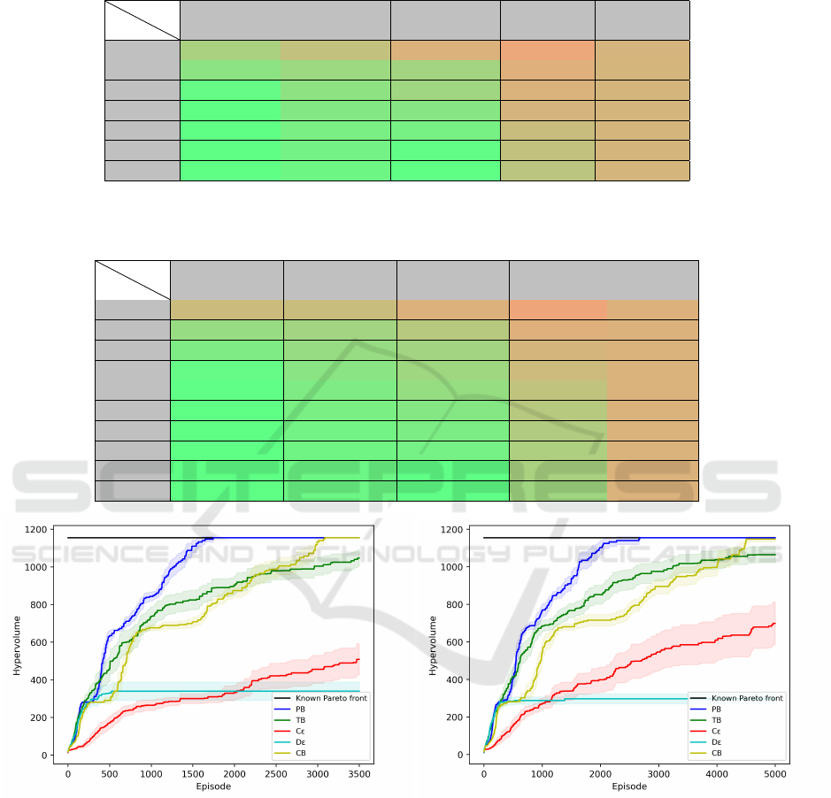
Table 2: Hypervolume mean and standard deviation from the vectors in the starting state for different strategies every 500

episodes on the DST. Bold ﬁgures signify the means are statistically different from the means of Cε and Dε according to

ANOVA and Turkey’s tests.

Eps.

Metas

PB TB CB Cε Dε

500 634.8 ± 92.8 460.9 ± 205.1 290.3 ± 58.4 170.4 ± 105.1 330.4 ± 10.7

1000 843.3 ± 76.1 736.3 ± 166.3 676.2 ± 46.8 264.8 ± 89.9 339.4 ± 144.1

1500 1110 ± 107.1 824.3 ± 167.3 703.8 ± 76.3 300.1 ± 83.2 339.6 ± 156.6

2000 1155 ± 0 903.9 ± 152 874.5 ± 117.5 333.1 ± 126.1 339.6 ± 157

2500 1155 ± 0 979.2 ± 153 987.6 ± 151.8 420.9 ± 215.5 339.6 ± 157

3000 1155 ± 0 1004.1 ± 154.8 1132.5 ± 79 455.7 ± 240.8 339.6 ± 157

3500 1155 ± 0 1047.6 ± 141.7 1155 ± 0 508.7 ± 269.2 339.6 ± 157

Table 3: Hypervolume mean and standard deviation from the vectors in the starting state for different strategies every 500

episodes on the MDST. Bold ﬁgures signify the means are statistically different from the means of Cε and Dε according to

ANOVA and Turkey’s tests.

Eps.

Metas

PB TB CB Cε Dε

500 405.1 ± 159.1 413.8 ± 169.9 281 ± 0 154.3 ± 102.9 284.1 ± 66.8

1000 765.3 ± 112.7 685.1 ± 96.8 542.1 ± 179.7 270.4 ± 94.2 287.3 ± 63.4

1500 937.5 ± 133.9 767.1 ± 119.6 680.8 ± 54.5 338.6 ± 154.8 296.7 ± 85.5

2000 1102.5 ± 114 852.2 ± 162.8 716.1 ± 100 398.4 ± 217.5 296.7 ± 85.5

2500 1140 ± 65.4 933.5 ± 172.4 771.3 ± 112.9 477.4 ± 262.5 296.7 ± 85.5

3000 1155 ± 0 975.4 ± 163.2 895.5 ± 126.8 545.9 ± 320 296.7 ± 85.5

3500 1155 ± 0 1017.9 ± 157.9 952.8 ± 151.6 584.8 ± 343.5 296.7 ± 85.5

4000 1155 ± 0 1037.7 ± 154.2 997.5 ± 149.8 609.4 ± 365.2 296.7 ± 85.5

4500 1155 ± 0 1056.3 ± 142.4 1140 ± 65.4 636 ± 372.6 296.7 ± 85.5

5000 1155 ± 0 1065 ± 137.5 1147.5 ± 46.8 698.8 ± 368.5 296.7 ± 85.5

Figure 6: Evolution of the hypervolume of the found poli-

cies during the training in the DST environment.

timal policies in the given training window. TB and

CB strategies are performing well when compared to

the two ε-greedy strategies but fail to ﬁnd all optimal

strategies.

In this scenario again, Dε stops ﬁnding new poli-

cies as it becomes greedier and lacks exploration. Fi-

nally, Cε behaves the same as in the other environ-

ment, i.e. it keeps learning new points with episodes,

but with a high variance.

Figure 7: Evolution of the hypervolume of the found poli-

cies during the training in the Mirrored DST environment.

As for the DST, Table 3 presents numerical results

of the experiments. The same conclusion as for the

DST holds; metaheuristics inspired approaches are

statistically better than state-of-the-art approaches on

this environment.

Metaheuristics-based Exploration Strategies for Multi-Objective Reinforcement Learning

671

6 CONCLUSION

In this paper, a framework for multi-policy inner-loop

MORL training has been presented. It is modular; it

allows to change some of its part without the need to

change the others. From that framework, the possibil-

ity to apply state-of-the-art optimization methods to

MORL was identiﬁed.

Three new exploration strategies were presented

to solve the exploration problem in this setting: Re-

pulsive Pheromones-based, Count-based and Tabu-

based. These are inspired from existing work in meta-

heuristics. All three proposed strategies perform bet-

ter than current state-of-the-art, ε-greedy based meth-

ods on the studied environments. Also, it is shown

that behavioral policies which do not converge to be-

come greedy perform better than converging ones in

the learning phase.

Because of the lack of benchmark environments,

this paper also proposes a new benchmark called the

Mirrored Deep Sea Treasure. It is a harder version of

the well known Deep Sea Treasure.

As future work, we plan to introduce new

(stochastic) benchmarks, use MORL algorithms to

control actual robots, and to continue to study the

application of traditional optimization techniques to

MORL.

ACKNOWLEDGEMENTS

This work is funded by the Fonds National de la

Recherche Luxembourg (FNR), CORE program un-

der the ADARS Project, ref. C20/IS/14762457.

REFERENCES

Amin, S., Gomrokchi, M., Satija, H., van Hoof, H., and

Precup, D. (2021). A Survey of Exploration Methods

in Reinforcement Learning. arXiv:2109.00157 [cs].

arXiv: 2109.00157.

Barrett, L. and Narayanan, S. (2008). Learning all opti-

mal policies with multiple criteria. In Proceedings of

the 25th international conference on Machine learn-

ing - ICML ’08, pages 41–47, Helsinki, Finland. ACM

Press.

Gambardella, L. M. and Dorigo, M. (1995). Ant-Q: A Re-

inforcement Learning approach to the traveling sales-

man problem. In Prieditis, A. and Russell, S., editors,

Machine Learning Proceedings 1995, pages 252–260.

Morgan Kaufmann, San Francisco (CA).

Hayes, C., R

adulescu, R., Bargiacchi, E., K

allstr

om, J.,

Macfarlane, M., Reymond, M., Verstraeten, T., Zint-

graf, L., Dazeley, R., Heintz, F., Howley, E., Irissap-

pane, A., Mannion, P., Nowe, A., Ramos, G., Restelli,

M., Vamplew, P., and Roijers, D. (2021). A Practi-

cal Guide to Multi-Objective Reinforcement Learning

and Planning.

Jumper, J., Evans, R., Pritzel, A., Green, T., Figurnov,

M., Ronneberger, O., Tunyasuvunakool, K., Bates, R.,

ıdek, A., Potapenko, A., Bridgland, A., Meyer, C.,

Kohl, S. A. A., Ballard, A. J., Cowie, A., Romera-

Paredes, B., Nikolov, S., Jain, R., Adler, J., Back, T.,

Petersen, S., Reiman, D., Clancy, E., Zielinski, M.,

Steinegger, M., Pacholska, M., Berghammer, T., Bo-

denstein, S., Silver, D., Vinyals, O., Senior, A. W.,

Kavukcuoglu, K., Kohli, P., and Hassabis, D. (2021).

Highly accurate protein structure prediction with Al-

phaFold. Nature, 596(7873):583–589.

Oliveira, T., Medeiros, L., Neto, A. D., and Melo, J. (2020).

Q-Managed: A new algorithm for a multiobjective re-

inforcement learning. Expert Systems with Applica-

tions, 168:114228.

Parisi, S., Pirotta, M., and Restelli, M. (2016). Multi-

objective Reinforcement Learning through Continu-

ous Pareto Manifold Approximation. Journal of Ar-

tiﬁcial Intelligence Research, 57:187–227.

Roijers, D. M., R

opke, W., Nowe, A., and Radulescu,

R. (2021). On Following Pareto-Optimal Policies in

Multi-Objective Planning and Reinforcement Learn-

ing.

Roijers, D. M., Vamplew, P., Whiteson, S., and Dazeley,

R. (2013). A survey of multi-objective sequential

decision-making. Journal of Artiﬁcial Intelligence Re-

search, 48(1):67–113.

Ruiz-Montiel, M., Mandow, L., and P

erez-de-la Cruz, J.-

L. (2017). A temporal difference method for multi-

objective reinforcement learning. Neurocomputing,

263:15–25.

Silver, D., Huang, A., Maddison, C. J., Guez, A., Sifre, L.,

van den Driessche, G., Schrittwieser, J., Antonoglou,

I., Panneershelvam, V., Lanctot, M., Dieleman, S.,

Grewe, D., Nham, J., Kalchbrenner, N., Sutskever, I.,

Lillicrap, T., Leach, M., Kavukcuoglu, K., Graepel,

T., and Hassabis, D. (2016). Mastering the game of

Go with deep neural networks and tree search. Na-

ture, 529(7587):484–489.

Sutton, R. S. and Barto, A. G. (2018). Reinforcement Learn-

ing: An Introduction. Adaptive Computation and Ma-

chine Learning series. A Bradford Book, Cambridge,

MA, USA, 2 edition.

Talbi, E.-G. (2009). Metaheuristics: From Design to Imple-

mentation, volume 74.

Vamplew, P., Dazeley, R., Berry, A., Issabekov, R., and

Dekker, E. (2011). Empirical evaluation methods

for multiobjective reinforcement learning algorithms.

Machine Learning, 84(1):51–80.

Vamplew, P., Dazeley, R., and Foale, C. (2017a). Soft-

max exploration strategies for multiobjective rein-

forcement learning. Neurocomputing, 263:74–86.

Vamplew, P., Issabekov, R., Dazeley, R., Foale, C., Berry,

A., Moore, T., and Creighton, D. (2017b). Steering ap-

proaches to Pareto-optimal multiobjective reinforce-

ment learning. Neurocomputing, 263:26–38.

ICAART 2022 - 14th International Conference on Agents and Artiﬁcial Intelligence

672

Van Moffaert, K., Drugan, M. M., and Now

e, A. (2013).

Hypervolume-Based Multi-Objective Reinforcement

Learning. In Purshouse, R. C., Fleming, P. J., Fon-

seca, C. M., Greco, S., and Shaw, J., editors, Evolu-

tionary Multi-Criterion Optimization, Lecture Notes

in Computer Science, pages 352–366, Berlin, Heidel-

berg. Springer.

Van Moffaert, K. and Now

e, A. (2014). Multi-objective re-

inforcement learning using sets of pareto dominating

policies. The Journal of Machine Learning Research,

15(1):3483–3512. Publisher: JMLR. org.

Wang, W. and Sebag, M. (2013). Hypervolume indicator

and dominance reward based multi-objective Monte-

Carlo Tree Search. Machine Learning, 92(2):403–

429.

White, D. (1982). Multi-objective inﬁnite-horizon dis-

counted Markov decision processes. Journal of Math-

ematical Analysis and Applications, 89(2):639–647.

Wiering, M. A. and de Jong, E. D. (2007). Comput-

ing Optimal Stationary Policies for Multi-Objective

Markov Decision Processes. In 2007 IEEE Interna-

tional Symposium on Approximate Dynamic Program-

ming and Reinforcement Learning, pages 158–165.

ISSN: 2325-1867.

Wiering, M. A., Withagen, M., and Drugan, M. M. (2014).

Model-based multi-objective reinforcement learning.

In 2014 IEEE Symposium on Adaptive Dynamic Pro-

gramming and Reinforcement Learning (ADPRL),

pages 1–6, Orlando, FL, USA. IEEE.

Metaheuristics-based Exploration Strategies for Multi-Objective Reinforcement Learning

673