
Towards Depth Perception from Noisy Camera based Sensors for
Autonomous Driving
Mena Nagiub
1
and Thorsten Beuth
2
1
Valeo Schalter und Sensoren GmbH, Bietigheim-Bissingen, Germany
2
Valeo Detection Systems GmbH, Bietigheim-Bissingen, Germany
Keywords:
Monocular Depth Prediction, Dense Depth Completion, Noise, Camera-based Sensors, LIDAR.
Abstract:
Autonomous driving systems use depth sensors to create 3D point clouds of the scene. They use 3D point
clouds as a building block for other driving algorithms. Depth completion and prediction methods are used to
improve depth information and inaccuracy. Accuracy is a cornerstone of automotive safety. This paper studies
different depth completion and prediction methods providing an overview of the methods’ accuracies and use
cases. The study is limited to low-speed driving scenarios based on standard cameras and Laser sensors.
1 INTRODUCTION
The first step in autonomous driving is the environ-
ment perception with depth maps as an essential input
(Dijk and Croon, 2019). This study analysis achieve-
ments of deep learning for depth prediction, comple-
tion and noise improvement methods. The aim is to
define guidelines for designing a depth sensor or a fu-
sion of sensors for the safety of intended functions.
Depth perception is done using sensors like cam-
era, LIght Detection And Ranging (LIDAR), RA-
dio Detection And Ranging (RADAR), and ultrasonic
sensors. This study focuses on cameras and LIDARs.
Cameras suffer from noise when used for depth
preception (Bartoccioni et al., 2021), since distant ob-
jects are represented by less number of pixels, also
higher color variance leads to depth prediction er-
rors. Also, cameras are sensitive to: 1) calibration and
alignment, 2) sharp edges, causing blurriness, 3) am-
bient light, 4) rough weather conditions, and 5) col-
ors, textures, and shades.
Monocular depth estimation using motion (optical
flow) suffer from additional problems as absence of
relative motion between consecutive frames results in
worse depth accuracy, up to a complete failure. Be-
sides, this methods demand objects to move with a
non-zero relative speed (Watson et al., 2021).
LIDARs are considered as the most accurate
method for creating 3D maps (Chen et al., 2018).
They are impacted by (Sjafrie, 2019): 1) multi-path
reflections, 2) terrible weather conditions, and 3) ma-
terial reflection factor. Especially sparse LIDARs suf-
fer from: 1) rolling shutter effects, 2) irregular distri-
bution of sparse point cloud, and 3) dropped points or
incorrect distance calculations.
In section 2, we will focus on modern deep learn-
ing methods for depth maps completion and predic-
tion and noise improvements. section 3 is a compara-
tive study between the selected methods, and section
4 provides a conclusion and outlook.
2 DEEP LEARNING METHODS
Deep learning methods for depth completion and pre-
diction can be classified by: 1) tackled use cases, 2)
used architectures, and 3) noise tackling methods.
Supervised training is used when enough ground
truth data is available. When there is no ground truth,
other methods like semi-supervised, self-supervised,
or unsupervised training methods are used.
2.1 Tackled Use Cases
Use cases of depth perception can be classified into
sparse 3D point cloud completion and depth predic-
tion (or estimation) from 2D frames.
2.1.1 Sparse Point Cloud Completion
Fusion between sparse point cloud from LIDAR and
an additional monocular standard camera frame is the
primary trend for the depth completion.
198
Nagiub, M. and Beuth, T.
Towards Depth Perception from Noisy Camera based Sensors for Autonomous Driving.
DOI: 10.5220/0010989800003191
In Proceedings of the 8th International Conference on Vehicle Technology and Intelligent Transport Systems (VEHITS 2022), pages 198-207
ISBN: 978-989-758-573-9; ISSN: 2184-495X
Copyright
c
2022 by SCITEPRESS – Science and Technology Publications, Lda. All rights reserved

Camera frames act as an additional dense informa-
tion source to complete the sparse point cloud. The
camera can be used during the training phase as well
as the prediction phase through: 1) supervised learn-
ing method (Hu et al., 2021), (Qiu et al., 2019), (Xu
et al., 2019), (Li et al., 2020), (Chen et al., 2019), 2)
or unsupervised learning method (Ma et al., 2019),
(Shivakumar et al., 2019), (Park et al., 2020), (Wong
et al., 2020), (Van Gansbeke et al., 2019), (Cheng
et al., 2019), (Zhang et al., 2019)
2.1.2 Depth Prediction From Single Camera
Standard RGB cameras provide 2D frames with no
depth information. Systems can predict dense depth
map from camera frames with the support of infor-
mation from sparse LIDAR, where the camera is con-
sidered as the main source of the dense depth map,
while LIDAR sensor can be used in several ways: 1)
in training and prediction phases (Fu et al., 2020).
Training is done using supervised learning method
based on LIDAR accurate depth data. 2) In the train-
ing phase but not during prediction. Training is done
using the supervised learning method (Kumar et al.,
2018) using LIDAR data as ground truth. 3) In the
training phase but not during prediction. Training is
done using semi-supervised or self-supervised learn-
ing methods. Semi / self-supervised training is bene-
ficial when the LIDAR data is very sparse, not enough
to cover the whole field of view of the camera frame
(Bartoccioni et al., 2021).
Also, systems can predict dense depth map from
a standard RGB camera using information from an
additional stereo camera to be used only during the
training phase. The training can be done in super-
vised learning (Godard et al., 2019) or unsupervised
learning (Godard et al., 2017).
Some systems use other single-source dense depth
prediction methods when it is impossible to have a
sensor fusion. There are several methods to handle
this case: 1) a method uses a ground truth dense depth
map only during the training phase using a super-
vised learning method (Aich et al., 2021), (Kim et al.,
2020), (Fu et al., 2018), (Bhat et al., 2021). 2) Also
methods use information from a sequence of images
only during the training phase. Training is done using
a semi-supervised or self-supervised learning meth-
ods (Kumar et al., 2020), (Watson et al., 2021), (John-
ston and Carneiro, 2020).
2.2 Used Architectures
Most depth prediction and completion models are
based on the CNN features extraction block, which
Encoder: Features
Extraction
Decoder: Output
Decoding
Latent space,
Bottleneck
Input
Output
Copy / skip connection
Encoder Stage
Input
.
.
.
.
.
.
Decoder Stage
Input
.
.
.
.
.
.
conv 3 x 3 + ReLU
Max Pool 2 x 2
Copy conv 1 x 1
Transposed Conv 2 x 2
Copy conv 1 x 1
Figure 1: UNet / Encoder-Decoder with skip connections.
extracts depth clues from the raw sensors’ inputs to
build higher dimension features; this CNN is called
the encoder. The encoder’s last stage generates high
dimension features, also called the bottleneck, fol-
lowed by a prediction head that can predict the dense
depth map from the extracted features, also called the
decoder.
The mainstream trend uses UNet network (Ron-
neberger et al., 2015), refer to Figure 1. The encoder
side of UNet is usually replaced by VGG network (Si-
monyan and Zisserman, 2014) or ResNet network (He
et al., 2016). ResNet is preferred since it is config-
urable, replacing max-pooling layers with convolu-
tion kernels with longer strides to improve features
extraction. Recently EfficientNet network (Tan and
Le, 2019) has started to replace ResNet for the en-
coder side due to its reduced number of parameters.
The decoder side is often handcrafted according to the
required depth prediction method. The encoder and
decoder are often connected through skip connections
to improve prediction results through passing higher
resolution lower dimension features from the encoder
to the decoder. Some architectures use Conditional
Random Fields (CRF) (Liu et al., 2015) as a predic-
tion head (i.e., decoder) for the dense depth maps.
Features extraction blocks can be a dense CNN
(Watson et al., 2021), (Fu et al., 2020), (Chen et al.,
2019), (Fu et al., 2018) or cascaded CNN networks
(Aich et al., 2021), (Kumar et al., 2018). The pre-
diction heads can be as well upsampling transposed
convolution layers (Johnston and Carneiro, 2020)
or dense cascaded hourglass layers (i.e., encoder-
decoder with smaller scale) (Li et al., 2020).
Overall, architectures can be subdivided into late-
stage sensor fusion, early-stage sensor fusion, and
single sensor depth predictions architectures.
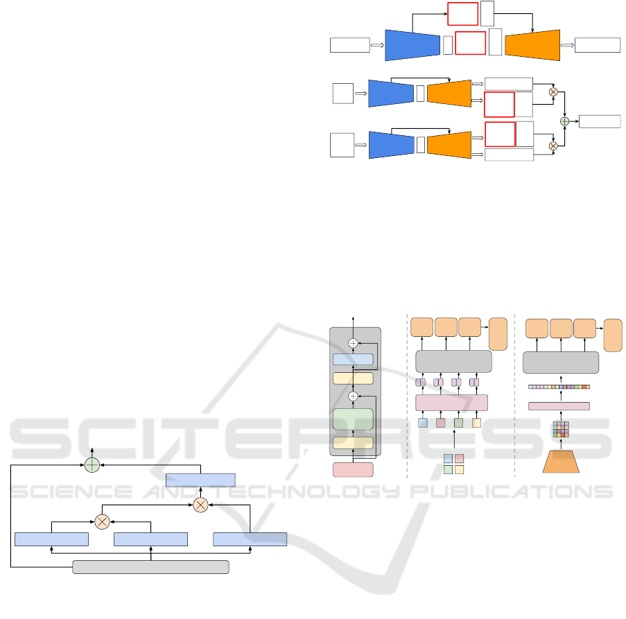
2.2.1 Late Stage Sensor Fusion Architectures
Late-stage sensor fusion architectures assume that
each sensor has an encoder branch up to the bottle-
neck stage, Figure 2. They are preferred over early-
stage sensor fusion architectures when the system’s
use case assumes the usage of different sensors as it
resolves the noise and errors of each sensor through
Towards Depth Perception from Noisy Camera based Sensors for Autonomous Driving
199

higher dimension feature fusion at the decoder side.
RGB Input
Point Cloud
Input
Dense
Depth Map
Encoder
Decoder
Encoder
Fusion and
Additional
Functionality
Block
RGB Input
Point Cloud
Input
Dense Depth
Map
Encoder
Decoder
Encoder
Coarse
Depth
RGB Input
Point Cloud
Input
Refined
Dense
Depth Map
Encoder
Encoder
Decoder
Decoder
Fusion and
Additional
Functionality
Block
Coarse
Depth
RGB Input
Point Cloud
Input
Dense
Depth Map
Fusion
Block
(a) Late fusion at the decoder input
(b) Late fusion of double branches at the decoder stages
(c) Late fusion of double branches at the decoder output
(d) Late fusion of cascaded multiscale hourglasses
Figure 2: There are four sub-architectures. (a) Fusion at de-
coder input (Shivakumar et al., 2019), (Wong et al., 2020),
(Cheng et al., 2019) where each encoder branch generates
bottleneck highest dimension features, those are fused at the
decoder input. (b) Fusion of double branches at decoder
internal stages (Qiu et al., 2019) which assumes each sen-
sor has an encoder-decoder branch, with additional decoder
stages at the fusion level. (c) Fusion of double branches
at the decoder output (Hu et al., 2021) assumes each sensor
has a complete standalone encoder-decoder branch. (d) Late
fusion of cascaded multiscale hourglasses architecture (Lin
et al., 2020) which is similar to late fusion at the decoder
stages. This architecture is used to resolve the scale ambi-
guity or resolution mismatch between different sensors.
The difference between the sub-architectures is
based on the stage at which the fusion happens on
the decoder side, Figure 2 (a, b, c, and d). This ar-
chitecture often requires fewer parameters compared
to early fusion. On the other hand, implementation of
encoder branches for sparse point clouds using con-
volutions is not efficient as it is similar to convolv-
ing Dirac pulse with a convolution filter (Wong et al.,
2020).
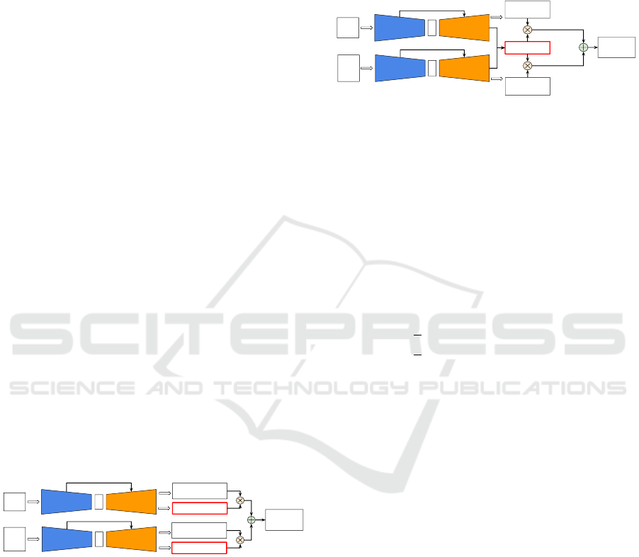
2.2.2 Early Stage Sensor Fusion Architectures
Early-stage sensor fusion is used when merged data
on raw format is required, compare Figure 3 (a, b, and
c). Processing raw data frames can miss high level
detailed features of each individual sensor.
RGB Image
LIDAR Point
Cloud
Dense Depth
Map
Encoder
Decoder
RGB Image
LIDAR Point
Cloud
Dense Depth
Map
Decoder
Fusion and
Additional
Functionality
Block
RGB Image
LIDAR Point
Cloud
Dense Depth
Map
Decoder
(a) Early fusion at the encoder input
(b) Early fusion using double branches at the encoder side
(c) Early fusion using double branches at the encoder stage
Figure 3: There are three sub architectures. (a) Fusion at
encoder input (Xu et al., 2019), (Park et al., 2020), (Zhang
et al., 2019) which fuses the input sensors’ data using sev-
eral methods like channel concatenation or data prepro-
cessing using a features extraction blocks. (b) Fusion us-
ing double branches (Wong et al., 2020) where each sen-
sor has a specific encoder branch followed by a functional
block, the bottleneck higher dimension features is an output
of the functional block. (c) Fusion using double branches
(Ma et al., 2019) where each sensor has a specific encoder
branch followed by several stages of the encoder. This kind
of fusion is also known as middle stage fusion.
2.2.3 Single Sensor based Architecture
This architecture is used with monocular RGB stan-
dard cameras. Training can be done with semi-
supervised learning where additional sensors could be
used to guide the learning process (Bartoccioni et al.,
2021) or in an unsupervised / self-supervised learning
method where a video sequence (Godard et al., 2019)
is used to build depth information over time.
Unsupervised / self-supervised learning methods,
as in Figure 4, do not need additional sensors, which
makes it cost-effective, but it requires additional mod-
ules for pose estimation, which requires additional
training.
Target frame
Additional
frame
Predicted Dense
Depth Map
Encoder
Pose
Estimation
Decoder
Photometric
Loss
Transformation
Matrix
Figure 4: General architecture for unsupervised monocular
dense depth prediction model.
Additional pose estimation module is used to esti-
mate the egomotion transformation matrix of the cam-
era due to the transformation from target frame image
t to a sequence frame either at instance t + 1 or at
instance t − 1 (Kumar et al., 2020). The pose estima-
tion module can be based on the Perspective-n-Point
(PnP) algorithm optimized using RANdom SAmple
Consensus (RANSAC). On the other hand, PoseNet
with 6 degrees of freedom (Kendall et al., 2015) can
VEHITS 2022 - 8th International Conference on Vehicle Technology and Intelligent Transport Systems
200
be used to estimate the pose. In either case, a relative
transformation matrix is estimated to define the trans-
formation from the target frame to the other frame.
2.3 Noise Tackling Methods
Noise and range uncertainty makes it challenging to
define an operational design domain for the sensor.
Hence, many state-of-the-art methods focus on tack-
ling noise and range accuracy to make the method
appealing for the automotive domain. Based on the
noise root cause, different methods are used to tackle
them.
2.3.1 Self-attention Blocks
Self attention block is based on the key-value-query
mechanism, Figure 5, (Jetley et al., 2018), (Wang
et al., 2018). The attention map A(ω) is calculated
from the input features map X(ω). The map gives a
global reference for each pixel, taking into account
feature similarity to surrounding pixels. The pre-
dicted target map is the weighted sum of all the input
pixels. Modern self-attention mechanisms replace the
CRF-based methods to capture global attention to the
details of the depth clues and can be integrated into
the architecture in different ways, Figure 6 (a and b).
Input Feature Map X(⍵): W ⨯ H ⨯ C
θ(Q): Conv(1 ⨯ 1) 𝜙(K): Conv(1 ⨯ 1) g(V): Conv(1 ⨯ 1)
Softmax
Conv (1 ⨯ 1)
Attention Map A(⍵) : W ⨯ H ⨯ C
Figure 5: Self attention blocks overall architecture.
2.3.2 Visual Transformers Encoder Blocks
Transformers are state-the-art method in natural lan-
guage processing (Jaderberg et al., 2015). They are
based on the advantages of the self-attention blocks
and residual blocks. Visual transformers (VisT) en-
coders are based on the encoder blocks of the trans-
formers. They can be used with raw images directly
or based on input coming from convolutional net-
works, which act as embeddings layers, Figure 7.
When used with raw images, then images need to be
patched and forwarded to an embedding layer which
transforms them into higher dimensional dense vec-
tors (Dosovitskiy et al., 2020).
Visual transformers encoders are used in the same
way as the self-attention blocks for capturing global
Input RGB
Image
Dense Depth
Map
Encoder Decoder
Self
Attention
Block
Attention
Map
Self
Attention
Block
Attention
Map
RGB
Input
Point
Cloud
Input
Coarse Dense
Depth Map
Encoder
Encoder
Decoder
Decoder
Coarse Dense
Depth Map
Self
Attention
Block
Attention
Map
Self
Attention
Block
Attention
Map
Refined Dense
Depth Map
(a) Self attention block for global context capture
(b) Self attention block for handling misalignment / sparsity
Figure 6: (a) Attention map is calculated and used as an ad-
ditional source of contextual features in addition to the fea-
tures extracted by other layers to support the dense depth es-
timation (Johnston and Carneiro, 2020), (Kim et al., 2020),
(Aich et al., 2021). (b) In case of solving sensor fusion
problems like misalignment or sparsity problems, attention
maps are used as a scoreboard. This scoreboard is used to
define the weight of fusion between different sensors’ out-
put features maps (Qiu et al., 2019).
L ⨯
MLP
Normalization
Multi-Headed
Attention
Normalization
Embedded
Patches
Transformer Encoder
Transformer Encoder
1 2 3 4
Linear Projection of Flattened
Patches
Patch +
Position
Embedding
MLP
Head
Class
Bird
Ball
Car
...
Attention
Head
Other
CNN
Raw Image
Flattened Layer
Transformer Encoder
MLP
Head
Class
Bird
Ball
Car
...
Attention
Head
Other
L ⨯
L ⨯
Figure 7: Visual transformer design and usage.
depth context cues. However, they require more pa-
rameters, and they are more complex to train (Bhat
et al., 2021). The added value of visual transform-
ers is that they provide higher dimension encoded fea-
tures that can be used by different decoders heads to
predict a different kind of information.
2.3.3 Spatial Propagation Networks
Spatial Propagation Networks (SPN) estimate miss-
ing values and refine less confident values by prop-
agating neighbors’ observations with corresponding
affinities (Park et al., 2020). In each iteration, the val-
ues of the pixels are improved based on affinity with
the neighbors using spatial propagation.
Spatial propagation solves the blurriness of the ob-
ject’s edges and inaccuracies due to the surface re-
flectiveness. SPN improves the depth accuracy of
inaccurate-depth points using the weighted sum of
the neighbor accurate-depth points. Accurate-depth
points can be detected from additional sources like
LIDAR measurements, while the less accurate-depth
points could be estimated depth points from the cam-
Towards Depth Perception from Noisy Camera based Sensors for Autonomous Driving
201
era (Hu et al., 2021), (Park et al., 2020).
2.3.4 Discrete Depth Volumes
Discrete depth volume is a technique to resolve the
depth measurements’ noise and ambiguities, either
due to the measurement accuracy or scale ambiguities
coming from the camera’s estimated depth. The goal
of the discretization is to convert the problem of the
continuous depth regression problem into a discrete
depth classification problem. First, the actual contin-
uous depth range is discretized into classes of depth
bins, and then the predicted depth is classified to be
assigned to one of these bins (Watson et al., 2021),
(Fu et al., 2018), (Bhat et al., 2021).
2.3.5 Confidence Maps
Confidence maps are used to handle uncertainty and
noise in the predicted dense depth maps. The basic
principle is to give a probability of the accuracy for
each predicted pixel. The confidence maps are usually
generated for less accurate sensors. First, the confi-
dence map is calculated as a weight for the predicted
depth accuracy of the pixel for each sensor. Then, the
predicted confidence map for each sensor is used as
weights for the depth value coming from that sensor
to calculate the final depth map.
There are no ground truth confidence maps, so
they are learned unsupervised. The whole system is
trained to predict the dense depth map compared to
the ground truth depth map. Figure 8 explains how
confidence maps are used inside the encoder-decoder
architecture (Hu et al., 2021), (Qiu et al., 2019), (Xu
et al., 2019), (Park et al., 2020), (Van Gansbeke et al.,
2019).
RGB
Input
Point
Cloud
Input
Coarse Dense Depth
Map
Encoder
Encoder
Decoder
Decoder
Confidence Map
Refined
Dense Depth
Map
Confidence Map
Coarse Dense Depth
Map
Figure 8: General architecture for confidence maps use
case.
2.3.6 Binary Masks
Binary masks are another technique similar to con-
fidence maps, but they are binary (0 or 1). They
are usually used to handle the problems related to
unavailable points in the sparse point cloud sensors
or the case of sensor fusion when there is an occlu-
sion in one sensor, which prevents it from predicting
the depth correctly. The binary mask is then used to
state whether the depth value in the final dense depth
map predicted by a certain sensor is to be used or
not. Binary masks are predicted by an unsupervised
method in the same way as confidence maps, or they
can be calculated using mathematical models. Figure
9 explains how confidence maps are used inside the
encoder-decoder architecture (Godard et al., 2019),
(Qiu et al., 2019), (Kumar et al., 2018).
RGB
Input
Point
Cloud
Input
Coarse Dense
Depth Map
Encoder
Encoder
Decoder
Decoder
Binary Mask
Refined
Dense Depth
Map
Coarse Dense
Depth Map
Figure 9: General architecture for binary masks use case.
2.4 Loss Functions
Loss functions have a significant role in the model’s
optimization to achieve the required accuracy (Zhao
et al., 2020), representing one way of noise tackling.
For the supervised learning L
1
loss function (i.e. ab-
solute mean error) and L
2
loss function (i.e. mean
square error) are usually used. The L
1s
smoothness
loss function in Eq. 1 improves learning process re-
sistance to outliers and exploding gradients.
L
1s
(d,
ˆ
d) =
(
1
N
∑
N
i=1
0.5 ·
ˆ
d
i
− d
i
2
, if
ˆ
d
i
− d
i
< 1
1
N
∑
N
i=1
ˆ
d
i
− d
i
− 0.5, otherwise
(1)
where N is the number of pixels per frame, d
i
the
predicted depth of pixel i for a specific training input
feature, and
ˆ
d
i
is the ground truth depth for the pixel.
The cross entropy loss function in Eq. 2 is used
with discrete classifications. For discrete depth vol-
umes and discrete bins, the loss function is used to
train the model for predicting the correct depth bin.
L
ce
(o) = −
N
∑
c=1
y
o,c
log(P
o,c
) (2)
where N is the number of possibly observed
classes, y
o,c
is a binary indicator (0 or 1), where it
is 1 if the class c is the correct classification for the
observation o, and P
o,c
is the predicted probability ob-
servation o is of class c.
The photometric loss function is uses a sequence
of frames to measure the quality of depth predictions
assuming that the camera moves between the frames
and is paired with unsupervised monocular depth es-
timation. The method requires a target frame at time
t and another sequence frame at time t + 1 or t − 1.
The depth will be predicted using the target frame.
The method then uses the predicted dense depth map,
the egomotion transformation matrix between the two
VEHITS 2022 - 8th International Conference on Vehicle Technology and Intelligent Transport Systems
202

consecutive frames, and the camera parameters to
project the target frame to reconstruct the sequence
frame according to Eq. 3
I
t→s
= I
s
h
proj(D
t
, T
t→s
, K)
i
(3)
where I
t→s
is the reconstructed sequence frame
from the targeted frame, I
s
is the sequence frame, D
t
is the depth map predicted from the target frame, T
t→s
is the relative egomotion transformation matrix from
the target frame to the sequence frame, K is the cam-
era intrinsic parameters matrix, and
h
.
i
is the element
wise sampling operator. So the photometric loss can
be calculated from the formula, Eq. 4,
L
pe
(I
s
, I
t→s
) =
α
2
(1 − SSIM(I
s
, I
t→s
))
+(1 − α)
|
I
s
− I
t→s
|
(4)
where L
pe
(I
s
, I
t→s
) is the photometric loss func-
tion between the sequence frame and the recon-
structed frame from the target frame to reconstruct
the sequence frame, I
t
is the target frame from which
depth map is predicted, I
t→s
is the reconstructed se-
quence frame from the target frame, SSIM() function
is structural similarity index between the sequence
frame and the reconstructed sequence frame, and α
is a weight parameter which is empirically chosen.
Egomotion CNN network can be trained to predict
the transformation matrix. Generally, if the prediction
is accurate, the predicted transformation matrix from
the sequence frame to the target frame will be the in-
verse matrix from the target to the sequence. In other
words, the multiplication of the two matrices should
result in an identity matrix. In this case, the formula
of the loss function, Eq. 5, is
L
ego
(I
s
, I
t
) = I − (T
s→t
· T
t→s
) (5)
where L
ego
(I
s
, I
t
) is the forward-backward egomo-
tion loss function between the target frame and the
sequence frame, T
t→s
is egomotion transformation
matrix from the target frame to the sequence frame,
T
s→t
is egomotion transformation matrix from the se-
quence frame to the target frame, and I is the identity
matrix.
Edge aware smoothness loss function L
es
(d)is
used to smooth the gradient calculation taking into
account the edges in the images; this ensures that the
depth is smoothed while pixels where the edges are
detected, the loss function will not consider them as
outliers. The formula for the loss function, Eq. 6, is
L
es
(d) =
1
N
N
∑
i=1
|∂
x
d
i
|e
|∂
x
I|
+ |∂
y
d
i
|e
|∂
y
I|
(6)
2.5 Model Training Methods
Dense depth perception tasks are very challenging,
especially for monocular cameras’ depth estimation.
The recorded image is ill-posed since a single 2D
frame can represent many different 3D projections.
For this reason, an extensive ground-truth dataset with
a massive number of examples is required to ensure
that the model is trained to solve the problem in su-
pervised learning correctly.
There are several challenges in building such a
ground truth dataset: 1) Amount of data sufficient,
enough to train the model parameters. 2) Cover many
different cases so that the model avoids overfitting. 3)
Cover the required use cases for the sensors used.
That is why it is not easy to build depth datasets,
and they are rare. Famous datasets like KITTI depth
benchmark dataset (Geiger et al., 2012), NYU-depth-
V2 dataset (Silberman et al., 2012), and Cityscape
dataset (Cordts et al., 2016) are available, but they are
not covering all required use cases.
2.6 Evaluation Metrics
Datasets are usually split into training and valida-
tion parts. The validation part is used for the accu-
racy benchmarking of the developed methods. Each
dataset provider defines certain metrics for the bench-
marking, but there are common metrics for evaluation
(Zhao et al., 2020), (Xiaogang et al., 2020) listed in
Table 1. The metric is calculated per frame, and then
it is averaged for the overall dataset. Where
ˆ
d
i
is the
ground truth depth for pixel i, d
i
is the predicted depth
of the pixel, and N is the total number of pixels in
the target frame. Inverse metrics are preferred to be
used, especially for depth prediction from a monocu-
lar camera, because it can handle infinite-depth prob-
lems, where depth value is undefined nor can be cal-
culated, resulting in infinite depth values.
3 COMPARATIVE STUDY
We have conducted a comparative study on some of
the most state-of-the-art methods validated using the
KITTI depth completion benchmark illustrating dif-
ferent use cases, architectures, and noise handling
methods. The methods are classified into depth pre-
diction from monocular cameras, Table 2, and depth
completion from sparse LIDAR and standard RGB
cameras fusion, Table 3. Figure 10 describes the ac-
curacy comparison between different monocular cam-
era depth prediction methods, measurements range
Towards Depth Perception from Noisy Camera based Sensors for Autonomous Driving
203
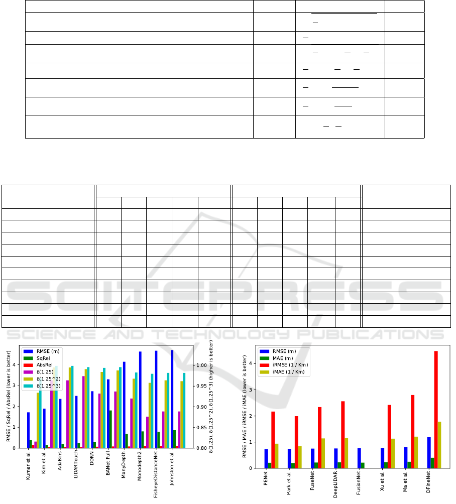
Table 1: Evaluation metrics.
Method description Abbr. Equation Unit
Root Mean Square Error (Lower the better)
RMSE
q
1
N
∑
N
i=1
(
ˆ
d
i
− d
i
)
2
mm
Mean Absolute Error (Lower the better)
MAE
1
N
∑
N
i=1
|
ˆ
d
i
− d
i
| mm
Inverse Root Mean Square Error (Lower the better)
iRMSE
q
1
N
∑
N
i=1
(
1
ˆ
d
i
−
1
d
i
)
2
1 / Km
Inverse Mean Absolute Error (Lower the better)
iMAE
1
N
∑
N
i=1
|
1
ˆ
d
i
−
1
d
i
| 1 / Km
Relative Squared Error (Lower the better)
SqRel
1
N
∑
N
i=1
(
ˆ
d
i
−d
i
)
2
(
ˆ
d
i
)
2
NA
Absolute Relative Difference (Lower the better)
AbsRel
1
N
∑
N
i=1
|
ˆ
d
i
−d
i
ˆ
d
i
| NA
Percentage of pixels satisfying accuracy thresholds(τ)
(Higher the better)
δ
τ
max(
ˆ
d
i
d
i
,
d
i
ˆ
d
i
) < τ NA
Table 2: Monocular camera depth prediction methods architecture comparison. Legend: (EA) EncDec with Atten, (EV)
EncDec with VisT, (EO) EncDec with Optical Flow, (CD) CNN / Deconv, (CCD) Cascaded CNN / Deconv, (SA) Self Atten-
tion Block, (VT) Visual Transformer, (DP) Discrete Depth Volume, (CM) Confidence Maps, (GT) LIDAR as ground truth
Method
Architecture Noise handling methods
Learning method
EA EV EO CD CCD SA VT DP CM GT
Kumar et al. X X X Supervised
Kim et al. X X Supervised
Adabins X X X Supervised
LIDARTouch X X Self-supervised
DORN X X Supervised
BANet Full X X Supervised
ManyDepth X X Self-supervised
Monodepth2 X Self-supervised
FisheyeDistanceNet X X Self-supervised
Johnston et al. X X X Self-supervised
Figure 10: Monocular camera depth prediction methods ac-
curacy comparison. The lower the RMSE value the better
the method accuracy.
from 0 m to 80 m, and Figure 11 describes the ac-
curacy comparison between different depth comple-
tion methods using sparse LIDAR and RGB standard
camera sensor fusion, measurements range from 5 m
to 180 m. We compare selected methods based on
Figure 11: Sparse LIDAR / Monocular camera fusion depth
completion methods accuracy comparison. The lower the
RMSE value the better the method accuracy.
Root Mean Square Error (RMSE) as it is a common
metric between all methods. For the monocular cam-
era depth prediction, the RMSE varies around a value
of 1.7 of up to 4.7 m. While for the depth com-
pletion using LIDAR and camera fusion, the RMSE
VEHITS 2022 - 8th International Conference on Vehicle Technology and Intelligent Transport Systems
204
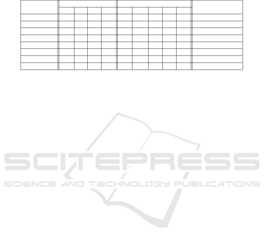
Table 3: Sparse LIDAR / Monocular camera fusion depth completion methods architecture comparison. Legend: (DB) Double
branch fusion, (DI) Decoder input fusion, (EF) Early input fusion, (CD) CNN / Deconv, (SA) Self Attention Block, (CM)
Confidence maps, (CS) CSPN, (EF) Extra Features Vectors, (GT) LIDAR as ground truth
Method
Architecture Noise handling methods
Learning method
DB DI EF CD SA CM CS EF GT
PENet X X X Supervised
Park et al. X X Unsupervised
FuseNet X Supervised
DeepLIDAR X X X X X Self-supervised
FusionNet X X Supervised
Xu et al. X X X X Supervised
Ma et al. X Self-supervised
DFineNet X Self-supervised
value varies around 0.73 up to 1.18 m. Thus, we can
hypothesize that the accuracy of LIDAR and Camera
fusion is better than monocular depth prediction.
3.1 Impact of Certain Architectures
In general we can interpret from the comparisons (Ta-
bles 2 and 3, and Figures 10 and 11) that for LIDAR
and Camera fusion, late stage sensor fusion archi-
tecture, e.g. (Hu et al., 2021), (Chen et al., 2019),
(Van Gansbeke et al., 2019), overall provide better
accuracy than early stage architectures; we hypothe-
size that accuracy is improved due to noise correction
by the encoder branch for each sensor. On the other
hand, for monocular camera depth encoder-decoder
architecture based methods, e.g. (Kim et al., 2020),
(Bhat et al., 2021), (Bartoccioni et al., 2021) provide
similar results to other dense CNN and cascaded CNN
methods, e.g. (Kumar et al., 2018), (Fu et al., 2018).
3.2 Impact of Noise Handling Methods
According to the study’s results, we hypothesize that
usage of LIDARs as ground truth improves the ac-
curacy; their higher accuracy helps models to learn
better parameters. Comparing (Kumar et al., 2018),
and (Bartoccioni et al., 2021) to other methods, shows
better accuracy which might be due to the usage of
LIDAR during training. Furthermore, we hypothe-
size that self-attention blocks and VisT encoders im-
prove the depth prediction since the attention maps
reflect the context of objects and their relative depth.
This could improve the depth maps, especially when
several objects have relatively different depth values.
For example, methods (Kim et al., 2020), (Bhat et al.,
2021) improve the accuracy by using attention maps,
also for DeepLIDAR method (Qiu et al., 2019) which
is using self-supervised training and has similar accu-
racy to PENet method (Hu et al., 2021). Furthermore,
we hypothesize that depth volume discretization im-
proves depth accuracy. The discretization might im-
prove the predicted depth by predefined depth bins,
which helps to constrain the predictions to predefined
scene ranges and remove inaccuracies due to noise.
Finally, We hypothesize that confidence maps im-
prove the accuracy since it is one of the methods to
learn the noise model itself, and hence it would help
compensate for the detected noise in prediction.
3.3 Impact of Training Methods
Based on Figures 10 and 11, supervised learning
methods show overall better performance. This con-
clusion aligns with the usage of LIDARs as ground
truth for monocular camera depth prediction since us-
ing accurate LIDARs would provide a similar effect
as round truth datasets.
4 CONCLUSION AND OUTLOOK
In this paper, we have shown how the usage of
dedicated noise handling blocks, supervised learn-
ing methods, and specific architectures in specific
cases can be used to design a depth perception sensor
with improved accuracy, leading to better operational
design domain (ODD) for the function of the au-
tonomous driving / advanced driving assistance sys-
tems. As an example, in the case of LIDAR-camera
sensor fusion, the usage of late fusion with double
branch architecture along with confidence maps im-
proves dense depth map completion in PENet (Hu
et al., 2021) (RMSE 0.73 m) compared to DFineNet
(Zhang et al., 2019) (RMSE 1.18 m) which uses early
fusion and no noise handling at all. On the other hand,
there is no clear favorable architecture for monocu-
lar camera depth prediction, but results show that us-
ing supervised learning methods and noise handling
techniques improves accuracy. As an example, (Ku-
mar et al., 2018) (RMSE 1.717 m), which uses LI-
Towards Depth Perception from Noisy Camera based Sensors for Autonomous Driving
205

DAR as ground truth for supervised learning, and
confidence maps, and uses cascaded CNN architec-
ture, outperforms FisheyeDistanceNet (Kumar et al.,
2020) (RMSE 4.669 m), which is trained unsuper-
vised and dependent on the encoder-decoder architec-
ture. Therefore, we can conclude that noise handling
methods improve the accuracy in all scenarios. Also,
model architecture is a critical factor of the sensor fu-
sion systems for depth completion tasks. In addition,
supervised learning through a dataset or an additional
accurate source provides better accuracy than other
learning methods.
The future trend of the safety of autonomous driv-
ing systems, especially depth perception systems, is
heading towards the definition of operational scenar-
ios and functional domains and validation and verifi-
cation architectures based on ODD to reduce uncer-
tainty as much as possible (Wiltschko et al., 2019).
ACKNOWLEDGEMENTS
We want to acknowledge the discussions with Mr.
Ganesh Sistu concerning the outlook section.
REFERENCES
Aich, S., Vianney, J. M. U., Islam, M. A., and Liu, M. K. B.
(2021). Bidirectional attention network for monocular
depth estimation. In 2021 IEEE International Con-
ference on Robotics and Automation (ICRA), pages
11746–11752. IEEE.
Bartoccioni, F., Zablocki,
´
E., P
´
erez, P., Cord, M., and
Alahari, K. (2021). Lidartouch: Monocular metric
depth estimation with a few-beam lidar. arXiv preprint
arXiv:2109.03569.
Bhat, S. F., Alhashim, I., and Wonka, P. (2021). Adabins:
Depth estimation using adaptive bins. In Proceedings
of the IEEE/CVF Conference on Computer Vision and
Pattern Recognition, pages 4009–4018.
Chen, Y., Tang, J., Jiang, C., Zhu, L., Lehtom
¨
aki, M.,
Kaartinen, H., Kaijaluoto, R., Wang, Y., Hyypp
¨
a, J.,
Hyypp
¨
a, H., et al. (2018). The accuracy compari-
son of three simultaneous localization and mapping
(slam)-based indoor mapping technologies. Sensors,
18(10):3228.
Chen, Y., Yang, B., Liang, M., and Urtasun, R. (2019).
Learning joint 2d-3d representations for depth com-
pletion. In Proceedings of the IEEE/CVF Interna-
tional Conference on Computer Vision, pages 10023–
10032.
Cheng, X., Zhong, Y., Dai, Y., Ji, P., and Li, H. (2019).
Noise-aware unsupervised deep lidar-stereo fusion. In
Proceedings of the IEEE/CVF Conference on Com-
puter Vision and Pattern Recognition, pages 6339–
6348.
Cordts, M., Omran, M., Ramos, S., Rehfeld, T., Enzweiler,
M., Benenson, R., Franke, U., Roth, S., and Schiele,
B. (2016). The cityscapes dataset for semantic urban
scene understanding. In Proceedings of the IEEE con-
ference on computer vision and pattern recognition,
pages 3213–3223.
Dijk, T. v. and Croon, G. d. (2019). How do neural net-
works see depth in single images? In Proceedings of
the IEEE/CVF International Conference on Computer
Vision, pages 2183–2191.
Dosovitskiy, A., Beyer, L., Kolesnikov, A., Weissenborn,
D., Zhai, X., Unterthiner, T., Dehghani, M., Minderer,
M., Heigold, G., Gelly, S., et al. (2020). An image is
worth 16x16 words: Transformers for image recogni-
tion at scale. arXiv preprint arXiv:2010.11929.
Fu, C., Dong, C., Mertz, C., and Dolan, J. M. (2020). Depth
completion via inductive fusion of planar lidar and
monocular camera. In 2020 IEEE/RSJ International
Conference on Intelligent Robots and Systems (IROS),
pages 10843–10848. IEEE.
Fu, H., Gong, M., Wang, C., Batmanghelich, K., and
Tao, D. (2018). Deep ordinal regression network
for monocular depth estimation. In Proceedings of
the IEEE conference on computer vision and pattern
recognition, pages 2002–2011.
Geiger, A., Lenz, P., and Urtasun, R. (2012). Are we ready
for autonomous driving? the kitti vision benchmark
suite. In 2012 IEEE conference on computer vision
and pattern recognition, pages 3354–3361. IEEE.
Godard, C., Mac Aodha, O., and Brostow, G. J. (2017).
Unsupervised monocular depth estimation with left-
right consistency. In Proceedings of the IEEE con-
ference on computer vision and pattern recognition,
pages 270–279.
Godard, C., Mac Aodha, O., Firman, M., and Brostow, G. J.
(2019). Digging into self-supervised monocular depth
estimation. In Proceedings of the IEEE/CVF Interna-
tional Conference on Computer Vision, pages 3828–
3838.
He, K., Zhang, X., Ren, S., and Sun, J. (2016). Deep resid-
ual learning for image recognition. In Proceedings of
the IEEE conference on computer vision and pattern
recognition, pages 770–778.
Hu, M., Wang, S., Li, B., Ning, S., Fan, L., and Gong,
X. (2021). Penet: Towards precise and efficient
image guided depth completion. arXiv preprint
arXiv:2103.00783.
Jaderberg, M., Simonyan, K., Zisserman, A., et al. (2015).
Spatial transformer networks. Advances in neural in-
formation processing systems, 28:2017–2025.
Jetley, S., Lord, N. A., Lee, N., and Torr, P. H. (2018). Learn
to pay attention. arXiv preprint arXiv:1804.02391.
Johnston, A. and Carneiro, G. (2020). Self-supervised
monocular trained depth estimation using self-
attention and discrete disparity volume. In Proceed-
ings of the ieee/cvf conference on computer vision and
pattern recognition, pages 4756–4765.
Kendall, A., Grimes, M., and Cipolla, R. (2015). Posenet: A
convolutional network for real-time 6-dof camera re-
VEHITS 2022 - 8th International Conference on Vehicle Technology and Intelligent Transport Systems
206

localization. In Proceedings of the IEEE international
conference on computer vision, pages 2938–2946.
Kim, D., Lee, S., Lee, J., and Kim, J. (2020). Leverag-
ing contextual information for monocular depth esti-
mation. IEEE Access, 8:147808–147817.
Kumar, V. R., Hiremath, S. A., Bach, M., Milz, S., Witt,
C., Pinard, C., Yogamani, S., and M
¨
ader, P. (2020).
Fisheyedistancenet: Self-supervised scale-aware dis-
tance estimation using monocular fisheye camera for
autonomous driving. In 2020 IEEE international con-
ference on robotics and automation (ICRA), pages
574–581. IEEE.
Kumar, V. R., Milz, S., Witt, C., Simon, M., Amende,
K., Petzold, J., Yogamani, S., and Pech, T. (2018).
Monocular fisheye camera depth estimation using
sparse lidar supervision. In 2018 21st Interna-
tional Conference on Intelligent Transportation Sys-
tems (ITSC), pages 2853–2858. IEEE.
Li, A., Yuan, Z., Ling, Y., Chi, W., Zhang, C., et al. (2020).
A multi-scale guided cascade hourglass network for
depth completion. In Proceedings of the IEEE/CVF
Winter Conference on Applications of Computer Vi-
sion, pages 32–40.
Lin, J.-T., Dai, D., and Van Gool, L. (2020). Depth estima-
tion from monocular images and sparse radar data. In
2020 IEEE/RSJ International Conference on Intelli-
gent Robots and Systems (IROS), pages 10233–10240.
IEEE.
Liu, F., Shen, C., Lin, G., and Reid, I. (2015). Learning
depth from single monocular images using deep con-
volutional neural fields. IEEE transactions on pat-
tern analysis and machine intelligence, 38(10):2024–
2039.
Ma, F., Cavalheiro, G. V., and Karaman, S. (2019). Self-
supervised sparse-to-dense: Self-supervised depth
completion from lidar and monocular camera. In 2019
International Conference on Robotics and Automation
(ICRA), pages 3288–3295. IEEE.
Park, J., Joo, K., Hu, Z., Liu, C.-K., and So Kweon, I.
(2020). Non-local spatial propagation network for
depth completion. In Computer Vision–ECCV 2020:
16th European Conference, Glasgow, UK, August 23–
28, 2020, Proceedings, Part XIII 16, pages 120–136.
Springer.
Qiu, J., Cui, Z., Zhang, Y., Zhang, X., Liu, S., Zeng, B., and
Pollefeys, M. (2019). Deeplidar: Deep surface normal
guided depth prediction for outdoor scene from sparse
lidar data and single color image. In Proceedings of
the IEEE/CVF Conference on Computer Vision and
Pattern Recognition, pages 3313–3322.
Ronneberger, O., Fischer, P., and Brox, T. (2015). U-net:
Convolutional networks for biomedical image seg-
mentation. In International Conference on Medical
image computing and computer-assisted intervention,
pages 234–241. Springer.
Shivakumar, S. S., Nguyen, T., Miller, I. D., Chen, S. W.,
Kumar, V., and Taylor, C. J. (2019). Dfusenet: Deep
fusion of rgb and sparse depth information for image
guided dense depth completion. In 2019 IEEE In-
telligent Transportation Systems Conference (ITSC),
pages 13–20. IEEE.
Silberman, N., Hoiem, D., Kohli, P., and Fergus, R. (2012).
Indoor segmentation and support inference from rgbd
images. In European conference on computer vision,
pages 746–760. Springer.
Simonyan, K. and Zisserman, A. (2014). Very deep con-
volutional networks for large-scale image recognition.
arXiv preprint arXiv:1409.1556.
Sjafrie, H. (2019). Introduction to Self-Driving Vehicle
Technology. Chapman and Hall/CRC.
Tan, M. and Le, Q. (2019). Efficientnet: Rethinking model
scaling for convolutional neural networks. In Interna-
tional Conference on Machine Learning, pages 6105–
6114. PMLR.
Van Gansbeke, W., Neven, D., De Brabandere, B., and
Van Gool, L. (2019). Sparse and noisy lidar comple-
tion with rgb guidance and uncertainty. In 2019 16th
international conference on machine vision applica-
tions (MVA), pages 1–6. IEEE.
Wang, X., Girshick, R., Gupta, A., and He, K. (2018). Non-
local neural networks. In Proceedings of the IEEE
conference on computer vision and pattern recogni-
tion, pages 7794–7803.
Watson, J., Mac Aodha, O., Prisacariu, V., Brostow, G., and
Firman, M. (2021). The temporal opportunist: Self-
supervised multi-frame monocular depth. In Proceed-
ings of the IEEE/CVF Conference on Computer Vision
and Pattern Recognition, pages 1164–1174.
Wiltschko, T. et al. (2019). Safety first for automated driv-
ing. Technical report, Daimler AG.
Wong, A., Fei, X., Tsuei, S., and Soatto, S. (2020).
Unsupervised depth completion from visual inertial
odometry. IEEE Robotics and Automation Letters,
5(2):1899–1906.
Xiaogang, R., Wenjing, Y., Jing, H., Peiyuan, G., and Wei,
G. (2020). Monocular depth estimation based on deep
learning: A survey. In 2020 Chinese Automation
Congress (CAC), pages 2436–2440. IEEE.
Xu, Y., Zhu, X., Shi, J., Zhang, G., Bao, H., and Li,
H. (2019). Depth completion from sparse lidar data
with depth-normal constraints. In Proceedings of the
IEEE/CVF International Conference on Computer Vi-
sion, pages 2811–2820.
Zhang, Y., Nguyen, T., Miller, I. D., Shivakumar, S. S.,
Chen, S., Taylor, C. J., and Kumar, V. (2019).
Dfinenet: Ego-motion estimation and depth refine-
ment from sparse, noisy depth input with rgb guid-
ance. arXiv preprint arXiv:1903.06397.
Zhao, C., Sun, Q., Zhang, C., Tang, Y., and Qian, F. (2020).
Monocular depth estimation based on deep learning:
An overview. Science China Technological Sciences,
pages 1–16.
Towards Depth Perception from Noisy Camera based Sensors for Autonomous Driving
207
