Performance of Databases Used in Data Stream Processing Environments

Manuel Weißbach and Thomas Springer

Faculty of Computer Science, Technische Universit

at Dresden, Germany

Keywords:

Stream Processing, Benchmarking, Database Benchmark, Big Data, Performance.

Abstract:

Data stream processing (DSP) is being used in more and more ﬁelds to process large amounts of data with min-

imal latency and high throughput. In typical setups, a stream processing engine is combined with additional

components, especially database systems to implement complex use cases, which might cause a signiﬁcant

decrease of processing performance. In this paper we examine the speciﬁc data access patterns caused by

data stream processing and benchmark database systems with typical use cases derived from a real-world

application. Our tests involve popular databases in combination with Apache Flink to identify the system

combinations with the highest processing performance. Our results show that the choice of a database is

highly dependent on the data access pattern of the particular use case. In one of our benchmarks, we found a

throughput difference of a factor of 46.2 between the best and the worst performing database. From our expe-

rience in implementing a complex real-world application, we have derived a set of performance optimization

recommendations to help system developers to select an appropriate database for their use case and to ﬁnd a

high-performing system conﬁguration.

1 INTRODUCTION

In almost all areas of the economy, digitization is

progressing rapidly. Larger and larger amounts of

data have to be processed in shorter and shorter pe-

riods of time. These data sets grow continuously, i.e.,

they are unbounded and thus, require new process-

ing paradigms since they are never completed. For

this purpose, Stream Processing Engines are often

adopted, that work according to the paradigm of Data

Stream Processing (DSP). Incoming data is processed

immediately upon arrival and thus remains in constant

ﬂow. This is also referred to as one-at-a-time process-

ing. In contrast to classic batch processing methods,

which collect data and process it in bursts, very low

processing latencies can be achieved.

Data stream processing architectures contain a

so called Data Stream Processing Engine (SPE) as

well as other components such as message queues

and databases. Although the latter contradicts the

paradigm of always keeping the data from the un-

bounded data stream ﬂowing (as described in (Stone-

braker et al., 2005)), the volumes of data to be pro-

cessed are in many cases too large to be kept in RAM,

so that the use of a persistence layer is unavoidable.

During our work on a research project in which

we process crowdsensed data of hundreds of thou-

sands of cyclists (partly live) using DSP, the inter-

action of the SPE and the database (DB) came into

our focus. In a ﬁrst performance study (Weißbach

et al., 2020) we analyzed the data management perfor-

mance of Cassandra, HBase, MariaDB, MongoDB,

and PostgreSQL while using them in combination

with the SPEs Apache Apex, Apache Flink, and

Apache Spark Streaming. The results clearly showed

that both, the choice of DB and the choice of SPE

have signiﬁcant impact on the overall processing per-

formance of the architecture. Apache Flink interacted

by far the best with the DBs systems we studied.

This ﬁnding led us to continue our implementations

based on this framework. With regard to the DB,

we did not get such a clear picture. Benchmark re-

sults appeared to be somewhat ”unpredictable” since

a database with superior performance in one experi-

ment often had a much worse performance in other

experiments. From the results we concluded that an

appropriate DB should be selected based on the most

frequently used access pattern generated by the spe-

ciﬁc use case and by the size of the data sets to be

processed. In addition, we derived the assumption,

that the algorithmic concepts used in Data Stream

Processing lead to particular query patterns when ac-

cessing the involved DB. These, however, are usually

not explicitly designed and optimized for use in DSP

Weißbach, M. and Springer, T.

Performance of Databases Used in Data Stream Processing Environments.

DOI: 10.5220/0011018300003200

In Proceedings of the 12th International Conference on Cloud Computing and Services Science (CLOSER 2022), pages 15-26

ISBN: 978-989-758-570-8; ISSN: 2184-5042

environments. As a consequence, the processing per-

formance of the DBs often falls short of expectations

while different component compositions of SPE and

DB interact better with each other than others. So

far, our research in (Weißbach et al., 2020) only cov-

ered binary, non-typed data management, in which the

DBs were only used as a pure storage medium and

not for data analysis. To ﬁnd out which DBs are best

suited with respect to our sensor data processing use

cases, we extended our benchmarking. In this paper,

we present our research results on typed data manage-

ment. Here, Apache Ignite, Cassandra, HBase, Mari-

aDB, MongoDB, and PostgreSQL as well as the in-

memory database Redis were included in the analysis.

In addition, the in-memory data grid Hazelcast was

tested as a cache and write buffer in combination with

Cassandra, HBase, MariaDB, MongoDB, and Post-

greSQL. All experiments were based on a DSP imple-

mentation for Apache Flink. During our work on this

topic, we made many optimizations to achieve solid,

high-performance data processing. At the end of the

paper, we want to pass on our resulting knowledge in

the form of recommendations for architecture design

to help developers to achieve their goals more quickly.

In summary, the following contributions are included

in this paper:

• We illustrate and characterize the typical access

patterns that arise from the use of windowing in

DSP processing.

• With benchmarks based on a real-world sen-

sor data processing use case we show which

databases achieved the best performance for dif-

ferent access types and discuss why.

• We make fundamental recommendations for

building a DSP architecture with an integrated

database.

The paper is organized as follows. In section 2

we present related work dealing with database bench-

marking and in section 3 the software systems used

in our experiments. In section 4 we characterize the

speciﬁc data access patterns we identiﬁed for DSP. In

section 5 we describe our benchmark setup and in sec-

tion 6 we present and interpret the benchmarking re-

sults. The lessons learned we derived from optimizing

our DSP architecture and the related benchmarks are

described in section 7. Finally, section 8 brieﬂy sum-

marizes the contents of the paper and provides infor-

mation on our plans to continue the research.

2 RELATED WORK

The performance of SQL and NoSQL databases for

Big Data processing has been investigated from vari-

ous perspectives. The Yahoo! Cloud Serving Bench-

mark (YCSB) (Cooper et al., 2010) is frequently used

to test storage solutions against predeﬁned workloads.

It is extensible in terms of workloads and connectors

to storage solutions and can therefore serve as a basis

for comparative benchmarks.

In (Cooper et al., 2010), YCSB was used to bench-

mark Cassandra, HBase, PNUTS, and MySQL as rep-

resentatives of DBs with different architectural con-

cepts. Hypothetical compromises derived from archi-

tecture decisions were conﬁrmed in practice. Cassan-

dra and HBase showed higher read latencies for high-

read workloads than PNUTS and MySQL, while the

update latencies for high-write workloads were lower.

While YCSB is designed to be extensible, the YCSB

client directly accesses the database interface layer.

Therefore, it does not provide facilities for an easy in-

tegration into a stream processing benchmark. Conse-

quently, we have implemented our own test environ-

ment.

The authors of (Abramova and Bernardino, 2013)

studied the impact of the data size on the query per-

formance of MongoDB and Cassandra in non-cluster

setups. A modiﬁed version of YCSB with six work-

loads was used. Their ﬁndings showed that as data

size increased, MongoDB’s performance decreased,

while Cassandra’s performance increased. In most

experiments, Cassandra performed better than Mon-

goDB.

In (Nelubin and Engber, 2013) a study of the per-

formance of Aerospike, Cassandra, MongoDB, and

Couchbase was presented with respect to the differ-

ences between using SSDs as persistent storage and

pure in-memory data management. They also used

the YCSB benchmark, with a cluster of four nodes.

Aerospike showed the best write performance in dis-

tributed use with SSDs with ACID guarantees ap-

plied. The authors themselves state, however, that

this result is partly due to the test conditions, which

matched the conditions for which Aerospike was op-

timized.

The performance of the distributed NoSQL

databases Cassandra, MongoDB, and Riak has been

investigated in (Klein et al., 2015). A setup of nine

production database servers optimized for processing

medical data with a high number of reads and updates

of single health records served as the basis for the

study. Different workloads were tested using YCSB

to collect results for both strong and eventual con-

sistency. Cassandra and Riak showed slightly lower

throughput for strong consistency (not all experiments

could be run for MongoDB). The Cassandra DB pro-

vided best overall performance in terms of throughput

in all experiments, but had the highest average access

CLOSER 2022 - 12th International Conference on Cloud Computing and Services Science

latencies.

In (Fiannaca, 2015) the authors investigated which

DB achieves the best throughput when querying

events from a robot execution log. They exam-

ined SQLite, MongoDB, and PostgreSQL, and rec-

ommended the use of MongoDB because of its good

throughput and usability for robot setups with a small

number of nodes or only a single node.

Cassandra, HBase, and MongoDB were bench-

marked in (Ahamed, 2016) with different cluster sizes

for various workloads. Cassandra consistently deliv-

ered the lowest access latency and highest throughput,

followed by HBase and MongoDB.

The performance of processing queries on

mobile users’ trajectory data was investigated

in(Niyizamwiyitira and Lundberg, 2017) using three

datasets from a telecom company. The study included

Cassandra, CouchDB, MongoDB, PostgreSQL, and

RethinkDB running on a cluster of four nodes

with four location-based queries and three datasets

of different sizes. Cassandra achieved the high-

est write throughput in distributed operation, while

PostgreSQL showed the lowest latency and highest

throughput in single-node setup. The lowest read la-

tency was achieved by MongoDB for all query types,

but it did not reach such a high throughput as Cassan-

dra. Furthermore, it was found that the read through-

put decreased with increasing data set size, especially

for random accesses.

While all studies examined the performance of

DBs in speciﬁc scenarios and domains, none of them

explicitly addressed how well they perform within

stream processing environments. To the best of our

knowledge, there are currently no studies that ex-

plicitly address this topic. However, such a context-

speciﬁc view is highly important as the data stream

processing leads to particular query patterns that may

have a signiﬁcant impact on the performance of the

DBs. Thus, our study is conducted to ﬁll this gap.

3 SOFTWARE

In the following, we introduce the used data stream

processing engine, Apache Flink, and the database

systems we studied.

Apache Flink is a DSP framework provided

under the Apache license 2.0 that supports batch

and stream processing in a hybrid fashion. Flink

implements data processing based on an operator

model that can be represented as a directed acyclic

graph. The individual operators can hold different

types of state information, depending on the require-

ments of the given use case, which is saved cyclically

using checkpointing based on a persistent storage

(e.g. HDFS or RocksDB). The operators of a Flink

application are executed in TaskSlots on worker

nodes, each of which has a TaskManager that handles

the node’s processing. For each application, there

is a JobManager that controls the execution of the

application and assigns corresponding tasks to the

TaskManagers. In order to run Flink highly available,

without a single point of failure, ZooKeeper is

additionally required. The service is used to store

status information of the JobManager so that it can

be replaced after a crash. Flink applications can op-

tionally be executed with at-most-once, at-least-once,

or exactly-once error semantics. For our use case, we

used exactly-once processing.

Apache Ignite is a distributed DB which was

designed for high-performance data analysis. Ignite

uses main memory as the primary storage medium

and thus enables particularly fast data accesses, since

there are no delays due to input and output operations

for ﬁxed memory access. The use of persistent mem-

ory is optional. In cluster mode, Ignite uses sharding

to distribute datasets managed as key-value pairs

among available nodes. The concept is based on the

so-called ”shared nothing architecture”, in which all

nodes of the cluster act completely independently and

can perform their own tasks without the involvement

of other nodes, since all the resources required are

available locally. Ignite clusters consist of two differ-

ent types of nodes, data nodes known as ”servers”,

that can manage data sets and indexes and perform

calculations on the data, and ”client” nodes, which

are used to establish connections between external

applications and the data servers. Data is distributed

across the cluster using the ”rendevouz” hashing

algorithm and, depending on the conﬁguration, may

be replicated as many times as desired or not at all.

When a node joins or leaves the cluster, the data is

rebalanced. Ignite provides various interfaces with

different abstraction levels, which can be used to

implement and use the DB in a variety of ways.

For example, it is possible to communicate with the

system on the basis of the SQL query language.

Apache Cassandra is a NoSQL DB that man-

ages data according to the ”wide-column store”

concept. Data is stored and queried based on a key-

value approach, whereby the data types of the stored

objects can differ. Cassandra was developed for high

scalability and reliability. Thus, the DB can manage

data volumes of several petabytes across several

thousand nodes and multiple data centers (Westoby,

Performance of Databases Used in Data Stream Processing Environments

2019). Cassandra supports various replication and

sharding methods in which the data is distributed to

the available nodes based on the hash sums of the

key values of the stored data. From client side, the

data can be managed using a custom query language

called ”Cassandra Query Language” (CQL), which is

similar to SQL.

Apache HBase is a non-relational DB devel-

oped as part of the Hadoop project that manages

data using Apache ZooKeeper and the Hadoop ﬁle

system HDFS. HBase can be seen as an abstraction

layer for HDFS that is intended to improve the

performance for particular record sizes and access

patterns. The processing approach is based on the

”big table” concept introduced by Google in (Chang

et al., 2008). The underlying ﬁle system, HDFS,

manages data in blocks of a ﬁxed size (64 MB by

default). This results in an inefﬁcient processing of

smaller data sets, which often arise in sensor data

management (our use case). HBase is optimized to

solve this problem by efﬁciently managing small sets

of data within large data volumes and by quickly

updating frequently changing data. An HBase cluster

consists of ”master”- and ”region”-servers. The

former coordinate data and task distribution using

ZooKeeper, the latter store data records, which are

logically divided into ”regions”. A region contains a

set of rows (DB entries) and is deﬁned according to

the range of key values of the contained entries. The

regions are distributed across multiple servers in the

cluster to achieve high read and write performance.

Thus, both sharding and replication of the data takes

place.

MariaDB is a relational DB that emerged as a

fork from MySQL. Since the most widely used Linux

distributions have replaced MySQL as the standard

DB with MariaDB, it is now considered more im-

portant by the open source community than MySQL,

which is not covered separately here. For distributed

operation, the software extension ”Galera” is used,

which replicates all data synchronously to all nodes

of the cluster (w/o sharding). There is no hierarchy

between the servers. Multi-master operation takes

place, in which both read and write requests can be

made to all servers. A MariaDB cluster manages data

in a transaction-safe manner according to the ACID

criteria. A quorum-based communication protocol

is used to ensure consistency. This means that the

system state is always assumed to be correct when

the majority of the servers in the cluster agree. To

avoid so-called ”split-brain” situations, in which half

of the servers agree to one of two different system

states, the number of nodes should always be odd

(2n + 1). In this case, up to n servers can fail at the

same time without any restrictions to the availability

of the cluster. If too many servers (more than n)

fail a majority decision is no longer possible and the

remaining servers will not answer any queries until at

least n + 1 servers are available again.

MongoDB is a non-relational, document-oriented

DB in which data is managed in JSON-like docu-

ments. The storage scheme allows the construction

of complex, nested data hierarchies, which can, how-

ever, be managed and queried in a clear and targeted

manner on the basis of indices. Data distribution

uses sharding and replication mechanisms. A cluster

consists of three different software components: the

”Mongos”, which distribute incoming requests, the

”Shards”, which manage so-called ”replica sets” and

the ”Conﬁg” server, which manages and provides

metadata for the cluster and conﬁguration for the

replica sets. A replica set contains a quantity of data

that is distributed to any number of shards. How

exactly the data is distributed can be freely conﬁg-

ured using the Conﬁg server and corresponding hash

functions. Incoming queries cannot be addressed

directly to the shards, but must always be forwarded

via the Mongos ﬁrst.

PostgreSQL, like MariaDB, is a classic relational

DB that processes data in a transaction-safe manner

according to the ACID principles. PostgreSQL can

be used as a DB cluster on the basis of a master-slave

approach, in which read queries can be made to all

nodes and write queries exclusively to the master

node, which thus represents a single point of failure.

Multi-master operation, similar to MariaDB, can be

enabled on the basis of (commercially distributed)

third-party extensions, but was not investigated in

this work.

Redis is an in-memory DB and therefore not

really suitable for our use case. Nevertheless, it can

be assumed that Redis achieves the best throughput

and latency values in all benchmarks or is only beaten

in this respect by DBs that also feature in-memory-

processing. Redis thus provides baseline values

for the metrics under consideration and shows the

costs of persistent data storage in comparison to the

other DBs. Redis manages data as key-value pairs.

The software runs in only one thread at a time and

thus does not take advantage of modern multi-core

processors. Redis can be operated as a DB cluster

with up to 1,000 nodes, with data distributed to the

nodes by means of sharding and replication.

CLOSER 2022 - 12th International Conference on Cloud Computing and Services Science

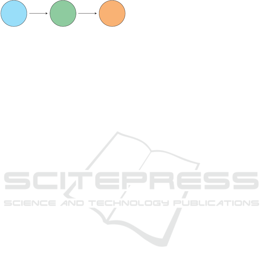
Generator Reducer Sink

keyBy

(+ windowing)

Figure 1: Operator graph of the test application.

Hazelcast is an in-memory data grid, i.e. a dis-

tributed system in which the nodes of the cluster

combine their available RAM virtually to enable

fast data exchange for applications without using

solid-state storage. Hazelcast can thus be used as

an in-memory DB. However, as practiced in this

study, it is also possible to implement Hazelcast as an

additional abstraction layer to extend an application

with a distributed cache for DB queries. For this

purpose Hazelcast provides appropriate programming

interfaces. These are used to deﬁne how the software

can persistently store data and load existing data. The

system can be combined with any data source, such as

DBs, ﬁle systems or REST interfaces. In the course

of implementing the application logic for a given use

case, there is no longer a direct connection to the DB

system used. Instead, all calls are handled via the

interfaces of Hazelcast, which maintains the loaded

DB contents in memory for fast access. Changes are

made in main memory and asynchronously persisted

in the connected DB. Hazelcast is highly scalable and

the architecture contains no single point of failure.

A variety of components are provided to integrate

Hazelcast into software projects. Hazelcast was

combined in this research series with all DBs that

do not provide main memory-based data processing

themselves (apart from query caches): Cassandra,

HBase, MariaDB, MongoDB and PostgreSQL.

4 DATABASE ACCESS PATTERNS

In this section we explore the speciﬁc data access pat-

terns that the concepts typically used in DSP generate

to the connected system components. This will be

demonstrated here brieﬂy with an example.

Figure 1 shows the operator pipeline of a simple

DSP application that produces data points in a gener-

ator and then groups them based on a key value con-

tained in these points. The reduce operator receives

multiple data points and combines them to a new data

point of the same object type. How the reduce op-

eration is implemented in detail is not important for

this example, but for instance, the data points could

contain integer values, which are simply summarized

by the reducer to create the resulting objects. Subse-

quently, the reduced data points are passed to a sink,

which persists the results (for example, by logging

them or writing them to a DB). This processing can

be optionally done with or without windowing.

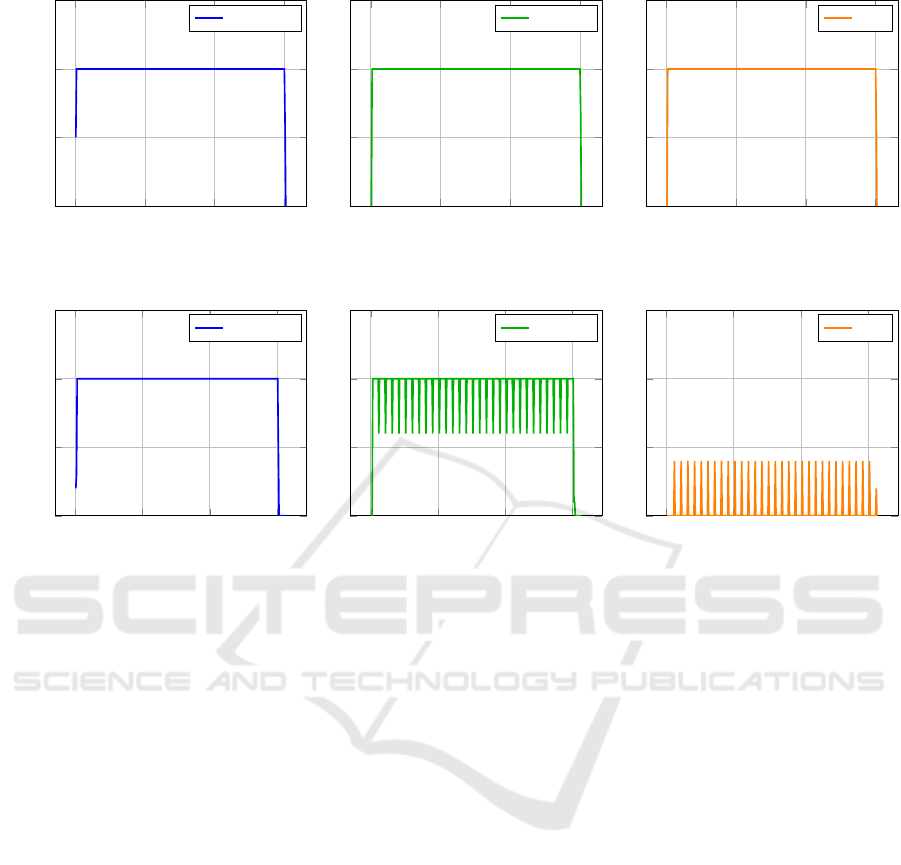
In our example, the generator was set to emit 100

data points per second. Figure 2 shows the result-

ing throughput for the three operators per tenth of a

second when no windowing is used. Figure 3 shows

the windowed version accordingly. There is no dif-

ference visible concerning the generator, but there is

for the reducer. If no windowing is used, the re-

ducer combines two input elements at a time and then

passes them on to the sink, which receives a stable

data stream. With windowing, the reducer does not

combine two elements at a time, but all elements of

the given window and outputs only one total result for

each window (here once per second). Depending on

the key distribution in the input data stream, there are

(few) less processing steps necessary, so the through-

put of the reducer drops at the end of each window

(every one second), which explains the cyclic pattern

in the ﬁgure. Consequently, the sink operator only

receives data points when the reducer has just com-

pleted a window, cyclically at intervals of one sec-

ond and idles the rest of the time. Considering that

each of the operators may access DBs and other ex-

ternal services, it becomes clear that the resulting re-

quest patterns are strongly inﬂuenced by the concepts

of DSP. In the present example, the windowing has

a great inﬂuence on the temporal distribution of the

accesses and it also leads to an aggregation of data

points. The keyBy() function as well as the amount

of different key values in the data stream also inﬂu-

ence the amount of elements arriving at the sink ev-

ery second and thus the number of write operations

triggered in a window. In conclusion, the access pat-

terns triggered by DSP processing are typically char-

acterized by cyclic accesses in which larger numbers

of requests are transmitted. If multiple processes, for

example windowing operations, are running in par-

allel, these patterns can overlap and possibly lead to

”chaotic” access sequences with poor resource uti-

lization and to race conditions. Since there are these

very special initial conditions for the use of DBs in

DSP applications, we decided to further investigate

their performance in a context-speciﬁc manner.

5 BENCHMARK SETUP

Our investigation included four complementary work-

loads with different DB access patterns, whose struc-

ture was based on a use case from our research

project, which is a typical real-world scenario from

the ﬁeld of sensor data analysis. Within this use case,

Performance of Databases Used in Data Stream Processing Environments

0 100 200 300

time (s/10)

processed elements

Generator

0 100 200 300

time (s/10)

Reducer

0 100 200 300

time (s/10)

Sink

Figure 2: Throughput of the generator, the reducer and the sink per tenth of a second when executed without windowing.

0 100 200 300

time (s/10)

processed elements

Generator

0 100 200 300

time (s/10)

Reducer

0 100 200 300

time (s/10)

Sink

Figure 3: Throughput of the generator, the reducer and the sink per tenth of a second when executed with windowing.

heat maps are generated and continuously updated

based on GPS measurements of cyclists. Municipal

trafﬁc planners from all over Germany can access the

maps using a web portal. The workloads were de-

signed to examine the performance of the DBs with

respect to speciﬁc access types (insert, update, ran-

dom read), as our previous research in (Weißbach

et al., 2020) showed that their performance usually

differs depending on these.

All experiments were performed on the server

cluster shown in ﬁgure 4, while taking care of an

equal technical baseline. Since the goal of the in-

vestigations was to ﬁnd out which DB is best suited

for our use case and interacts best with the chosen

SPE Apache Flink, the implementations used the pro-

vided DB interfaces that were best suited to build a

high-performance workﬂow. All system components

were conﬁgured according to the ofﬁcial instructions

and guidelines provided by their developers. Since

the DBs follow different data management concepts

and provide different interfaces, the implementation

variants differ to some extent.

The workloads are implemented in such a way that

the DB used (in the last operator) is always the slow-

est architectural component, making it the processing

bottleneck. Consequently, the DB controls the overall

throughput of the application by means of backpres-

sure mechanisms. This means the stream processing

engine adjusts the processing rates of the individual

operators to the maximum processing speed of the

slowest operator in the processing chain.

In the following sections, the four benchmarks are

described in detail.

Workload 1: Heatmap Generation

Figure 5 shows the operator pipeline of Workload

1. The implementation is based on the production

code of the use case. So-called ”trips” serve as input

data. Each trip contains the GPS points (recorded

with a frequency of 1 Hz) of a recorded bicycle ride

as well as metadata. For the benchmark, 14,409 trips

were exported into an efﬁciently readable binary ﬁle,

which is read in by the ”File Source” operator. The

MapToHeatmapCell operator calculates a geographic

hash value for each GPS point included in a trip and

emits a HeatmapCell object that assigns the number

of crossings made to this hash value (initial value: 1).

The data stream is grouped in the KeyByCellIndex

operator using the geographic hashes before the

HeatmapAggregation operator determines the total

number of crossings and updates the corresponding

value in the HeatmapCell object. The HeatmapEx-

porter stores the hash value, the crossings count, and

an event timestamp in the DB. Both the geographic

CLOSER 2022 - 12th International Conference on Cloud Computing and Services Science

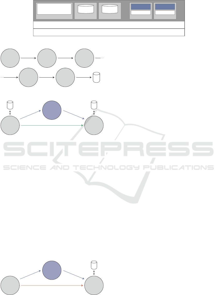
3 physical servers (24 core Intel Xeon Gold 6136, 354 GB RAM (DDR4), 500 GB NVME-SSD memory, 10GbE, Ubuntu 18.04.2 LTS)

Container

Monitoring:

Prometheus, Grafana,

Graphite

Docker Swarm

Container Container

…

DB DB

Container Container

Hadoop Hadoop

…

SPE SPE

Figure 4: Benchmark deployment.

File

Source

MapTo

HeatmapCell

KeyBy

CellIndex

Trip HeatmapCell

Heatmap

Aggregation

Heatmap

Exporter

HeatmapCellHeatmapCell

(windowing)

Figure 5: Operator graph for workload 1.

Reader

Window

Processing

Data

Management

Data (no windowing)

Data

(windowing)

Figure 6: Operator graph for workload 2.

hash and the timestamp are used as indexes. This

benchmark primarily provides information about

the application’s write performance during random

access.

Workload 2: Heatmap Copy

The second workload also examines the application’s

write performance, but with sequential access be-

havior. As shown in ﬁgure 6, an already existing

heatmap DB is read from a (PostgreSQL) source

DB and copied to the target DB. In total, the source

contains 418,239,564 entries.

Workload 3: Realistic Queries

Workload 3, shown in ﬁgure 7, examines the perfor-

mance of the system in querying the stored heatmap

information. For this purpose, a visualization tool

of the research project was modiﬁed to export all

DB queries into an efﬁciently readable binary data

format. The resulting ﬁle is used by the Flink

File

Source

Window

Processing

Data

Management

Queries (no windowing)

Queries

(windowing)

Figure 7: Operator graph for workloads 3 and 4.

application as a source dataset. It contains 1,292,600

entries generated by six users over a 10-hour usage

period. The dataset thus contains realistic query

patterns, which include a lot of duplicate queries, as

the users repeatedly viewed the same map sections in

the same resolution while working with the heat map.

The benchmark thus examines the performance of

the application in random data access, whereby an ef-

ﬁcient data caching yields large performance beneﬁts.

Workload 4: Random Queries

Workload 4 is similar to Workload 3, but the input

data set contains a randomly generated query pattern

without any duplicates. The benchmark examines the

read performance of the architecture when random

access is used, whereby data caching should not

provide notable performance beneﬁts.

6 BENCHMARK RESULTS

In total, we performed 152 experiments, in each of

which the processing time, the achieved throughput,

the end-to-end processing latency, the 95th percentile

of the processing latency, the DB access latency, the

95th percentile of the DB access latency, the CPU

utilization, the RAM utilization, the network utiliza-

tion as well as the persistent storage utilization re-

sulting from the experiments were measured. Due to

the amount of data and resulting diagrams, only those

metrics will be discussed in the following from which

relevant statements about the performance of the con-

sidered systems can be derived or which show note-

worthy peculiarities. Throughput values mentioned or

shown in the diagrams are mean values.

6.1 Preliminary Remarks

At this point, it should be noted once again that this

is not a ”classical” DB benchmark. The goal of the

study was to determine how good the tested DBs per-

form when they are used in a DSP environment and to

what extent they are suitable for sensor data process-

ing use cases. Consequently, the results presented in

the following provide information about the suitabil-

Performance of Databases Used in Data Stream Processing Environments

ity of the systems for this application area, but are not

representative for other ﬁelds.

6.2 Workload 1: Heatmap Generation

The diagram on the left in ﬁgure 8 shows the

throughput achieved when processing workload 1

with and without windowing. As expected, the Re-

dis in-memory DB achieves the highest throughput

(270,479 tuples/s). When processing the data with-

out windowing, the DBs achieved higher throughput

values when Hazelcast was used than when they were

operated individually. The effect can be explained by

the fact that Hazelcast already acknowledges the write

operations as successfully performed when the data

has been stored in main memory. The data is then

transferred to the underlying DBs asynchronously.

Hazelcast thus acts as a write buffer here, which is

beneﬁcial for the write throughput. It is also note-

worthy that Hazelcast achieves the highest throughput

with MariaDB (242,013 tuples/s), as exactly this DB

shows up the lowest throughput in standalone mode

(29,372 tuples/s). Hazelcast writes new data to the

connected DB cyclically every 5 seconds. Apparently,

the Galera-based MariaDB cluster copes much better

with this access pattern than with the original access

pattern of the streaming application. From this it can

be concluded that by using Hazelcast (or another in-

memory data grid) for buffering, a change in the write

pattern can be achieved, which can lead to higher pro-

cessing performance in DSP, since the pattern created

by the in-memory data grid is one that the DB can

better handle.

If windowing is used, the measurement results of

the system compositions with Hazelcast vary signif-

icantly. MongoDB even achieved worse throughput

values than in independent operation. The cause of

this behavior is the overlapping of the cyclic processes

of the DSP processing with the also cyclically per-

formed data write-out through Hazelcast. This results

in an inefﬁcient use of resources and sometimes full

utilization of the hardware.

Apart from the use of Hazelcast, PostgreSQL

(139,552 tuples/s without windowing, 110,905 tu-

ples/s with windowing), HBase (135,145 tuples/s w/o

w., 108,003 tuples/s w/ w.) and MongoDB (120,226

tuples/s w/o w., 82,950 tuples/s w/ w.) delivered the

best measurement results in both test variants. Cas-

sandra (41,626 tuples/s w/o w., 38,890 tuples/s w/

w.), Ignite (35,472 tuples/s w/o w., 33,780 tuples/s

w/ w.) and, as already mentioned, MariaDB (29,372

tuples/s w/o w., 32,363 tuples/s w/ w.) were far be-

hind. The comparatively low data throughput of Cas-

sandra is noteworthy to the extent that this DB de-

livered the best measured values when inserting and

updating small binary data sets in our previous study

(presented in (Weißbach et al., 2020)). This makes

clear that the results of these investigations cannot be

transferred to the management of typed data consid-

ered here.

6.3 Workload 2: Heatmap Copy

When copying the heatmap data, all DBs achieved

higher throughput values than in the heatmap gener-

ation with and without windowing, as the right dia-

gram in ﬁgure 8 shows. Accordingly, our measure-

ment results show that the processing latencies were

also lower for all DBs. This is due to the fact that the

data was processed sequentially, whereas the previ-

ous workload used random DB accesses. In addition,

only inserts (and no updates) were performed in this

benchmark.

Again, this access pattern shows large perfor-

mance differences in terms of processing with and

without windowing. As expected, Redis shows the

highest throughput and lowest latency values for

both variants. Omitting Redis, if no windowing is

used, the highest throughput values can be achieved

with Hazelcast for this experiment. The in-memory

data grid performed best in combination with HBase

(338,532 tuples/s). With windowing, a similar behav-

ior was observed with one exception (PostgreSQL).

The best measurement result in terms of throughput

was achieved by the combination of Hazelcast and

MariaDB (184,812 tuples/s).

When looking at the DBs in individual use, Post-

greSQL (189,542 tuples/s), MongoDB (133,005 tu-

ples/s) and HBase (106,869 tuples/s) generated the

highest throughput values without windowing in the

experiment variant. With windowing, the ranking

was quite similar: PostgreSQL (141,409 tuples/s),

HBase (120,690 tuples/s), MongoDB (87,379 tu-

ples/s). MariaDB, Cassandra and Ignite achieved

comparatively low throughput values.

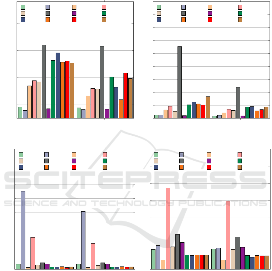
6.4 Workload 3 and 4: Realistic and

Random Queries

On the left, Figure 9 shows the throughput achieved

when processing real DB queries, and on the right, the

result for the randomized queries.

Two characteristics catch the eye immediately

when looking at the diagrams: Contrary to expecta-

tions, Redis did not achieve the highest measured val-

ues, and the results of the relational DBs PostgreSQL

and MariaDB stand out clearly. Both observations are

attributable to the number of accesses required for the

CLOSER 2022 - 12th International Conference on Cloud Computing and Services Science

without windowing with windowing

100

150

200

250

300

350

400

·10

41.627

38.890

29.372

32.363

1.2 · 10

82.950

1.4 · 10

1.11 · 10

1.35 · 10

1.08 · 10

2.7 · 10

2.66 · 10

35.472

33.780

2.13 · 10

1.53 · 10

2.42 · 10

1.15 · 10

2.07 · 10

68.911

2.11 · 10

1.67 · 10

2.03 · 10

1.48 · 10

average throughput in tuples/s

Cassandra

MariaDB MongoDB

PostgreSQL

HBase Redis Ignite

H+Cassandra

H+MariaDB H+MongoDB

H+PostgreSQL

H+HBase

without windowing with windowing

200

400

600

800

1.000

1.200

1.400

1.600

1.800

·10

53.474

38.848

52.934

46.856

1.33 · 10

87.379

1.9 · 10

1.41 · 10

1.07 · 10

1.21 · 10

1.11 · 10

4.81 · 10

42.501

40.550

2.12 · 10

1.74 · 10

2.52 · 10

1.85 · 10

2.26 · 10

1.17 · 10

2.08 · 10

1.38 · 10

3.39 · 10

1.72 · 10

average throughput in tuples/s

Cassandra

MariaDB MongoDB

PostgreSQL

HBase Redis Ignite

H+Cassandra

H+MariaDB H+MongoDB

H+PostgreSQL

H+HBase

Figure 8: Throughput achieved by the investigated databases for workload 1 (left) and workload 2 (right).

without windowing with windowing

·10

3.445

3.559

55.135

40.842

1.193

22.527

18.138

2.865

2.715

4.626

4.615

3.723

3.660

1.515

1.520

1.646

1.341

1.751

1.782

1.278

1.375

1.672

1.689

average throughput in tuples/s

Cassandra

MariaDB MongoDB

PostgreSQL

HBase Redis Ignite

H+Cassandra

H+MariaDB H+MongoDB

H+PostgreSQL

H+HBase

without windowing with windowing

·10

11.468

11.604

13.727

12.364

5.343

5.300

47.237

39.650

13.136

11.539

20.311

18.639

15.607

12.787

8.087

7.959

8.057

6.985

8.156

7.959

8.087

7.775

8.257

7.803

average throughput in tuples/s

Cassandra

MariaDB MongoDB

PostgreSQL

HBase Redis Ignite

H+Cassandra

H+MariaDB H+MongoDB

H+PostgreSQL

H+HBase

Figure 9: Throughput achieved by the investigated databases for workload 3 (left) and workload 4 (right).

data queries in particular. Each of the implementa-

tion variants was adapted to the conditions of the use

case and implemented and conﬁgured on the basis

of the ofﬁcial documentation and best practice pro-

cedures. However, the interfaces of the DBs differ

greatly. For example, most of the systems studied op-

erate on a key-value data management basis, where

access to multiple attributes usually requires multiple

DB queries. In addition, it is not possible in all DBs

to request multiple entries with a single query. With

relational DBs, which usually store individual entries

(table rows) as a contiguous data set, all required at-

tributes can be loaded with one read operation and

multiple queries can be made. This leads to a signiﬁ-

cant reduction of the DB queries, which is the reason

for the performance advantage of relational DBs.

A comparison of the two diagrams also makes

clear that the high processing performance of Mari-

aDB in the ﬁrst benchmark (55,135 tuples/s w/o w.,

40,842 tuples/s w/ w.) can be attributed to the efﬁ-

cient caching mechanisms of the DB. In the second

experiment, MariaDB’s throughput dropped signiﬁ-

Performance of Databases Used in Data Stream Processing Environments

cantly (13,727 tuples/s w/o w., 12,363 tuples/s w/ w.).

This collapse was not visible with PostgreSQL. Quite

the contrary, the DB even achieved higher through-

put values for the randomized queries. A possible

explanation for this is the ”pg prewarm” module that

PostgreSQL uses to reﬁll the data cache as quickly as

possible after a DB crash or restart. The module ﬁlls

the cache with information even before it has been

queried. This results in a signiﬁcant advantage in the

processing of randomized queries, even though they

do not contain any duplicates.

Apart from the relational DBs, the main memory-

oriented DBs Redis and Ignite performed best in

terms of throughput, followed by Cassandra and

HBase. MongoDB was the only DB that achieved

worse throughput when used individually than when

combined with Hazelcast. The use of Hazelcast does

not provide signiﬁcant beneﬁts for the present use

case. The additional processing steps required to load

data into memory are reﬂected in comparatively low

throughput values. Since the DBs under consideration

also feature main memory-based query caches them-

selves, they can achieve low response times. Hazel-

cast’s response times could be optimized by import-

ing the entire DB into main memory at the beginning.

In our setup, the caching is just done when the data

is accessed. However, due to the size of the DB, this

would result in a massive increase in the startup time

of the system, which would be undesirable for our use

case in production operation, especially during recov-

ery after the occurrence of an error.

6.5 Summary and Further Results

With regard to the benchmarks performed and the fur-

ther metrics recorded (but not illustrated here), the

following ﬁndings and observations can be noted:

• In the results presented, the implementation vari-

ants without windowing mostly achieved higher

throughput and lower latency values. This is due

to the structure of our benchmarking application.

It should not be wrongly concluded from this that

windowing generally slows down data processing.

• The use of Hazelcast results in higher throughput

and more stable processing for write access with-

out windowing in combination with most DBs

(except PostgreSQL). This can be explained by

the temporary data buffering in memory, which

decouples the writing of new data from the phys-

ical ﬁxed-memory access. However, if this effect

is intended to be utilized in an exactly-once appli-

cation, it is necessary to introduce safeguards that

ensure proper adherence to the semantics in the

event of Hazelcast failures.

• Using Hazelcast (or another in-memory data grid)

as a write buffer leads to a change in DB query

patterns. In some cases (see MariaDB), this

can contribute to a signiﬁcant increase in perfor-

mance, if it results in an access pattern that is

more suitable for the used DB than the one orig-

inally generated by the application logic. In con-

trast, PostgreSQL shows that there can be an in-

verse behavior, in which a DB is slowed down by

Hazelcast. Consequently, whether a performance

improvement can be achieved through the use of

Hazelcast must always be investigated on a use-

case- and access-pattern-speciﬁc basis.

• In terms of read access there were almost no ad-

vantages from using Hazelcast. The data sets used

in sensor data processing are usually of small size,

although they are queried en masse. Considering

that Hazelcast utilized a disproportionately large

amount of memory in our tests (signiﬁcantly more

than the size of the stored data sets and also more

than Redis required), it seems more appropriate

to operate the DBs under consideration without

the additional caching layer and to optimize their

own caching instead (with the help of appropriate

hardware resources).

• MariaDB had a very low CPU load and a high net-

work load while writing data in standalone mode.

This suggests that the overhead resulting from the

synchronous replication operations of the DB is

the cause of the low throughput values. When

combined with Hazelcast, resource utilization was

more in line with the other DBs. The collec-

tion and aggregation of write operations, which

are then performed in fewer DB queries (trans-

actions), leads to signiﬁcantly better performance

for the DB.

• PostgreSQL exhibited even higher network uti-

lization than MariaDB during writes. This can

also be explained by the data replication, which,

however, is done asynchronously and thus has less

of an impact on the system’s performance.

• HBase generated much greater disk usage than

the other DBs studied in all experiments. Post-

greSQL showed similar behavior, but only for

write queries and to a lesser extent. It can there-

fore be assumed that the performance of these sys-

tems is more dependent on the speed of the solid-

state storage used than that of the other systems,

which have fewer memory accesses.

• The in-memory DB Redis showed much higher

throughput values than the other DBs, especially

when writing data. This illustrates the massive

speed advantages resulting from the use of main

CLOSER 2022 - 12th International Conference on Cloud Computing and Services Science

memory for data processing. In the presented in-

vestigations, modern NVME SSDs were used as

data storage, which achieve a comparatively high

data throughput. It can be assumed that the gap

between Redis and the other DBs would be much

greater if classic hard disks had been used, which

are still the standard storage solution in most data

centers. This illustrates how important it is to

build a suitable storage hierarchy of fast ﬁxed stor-

age and large RAM-based DB caches.

7 LESSONS LEARNED

While working on these topics, we were frequently

challenged with various architectural design and com-

ponent conﬁguration problems that needed to be

solved in order to achieve high processing perfor-

mance. In the following, we present some approaches

that have been helpful in this regard:

• Architecture Components: To build a highly

available, fault-tolerant data stream processing

architecture, we recommend the use of Apache

Flink, Apache Kafka (as a buffer for incoming

messages), and a DB selected according to the re-

quirements of the use case. For ease of admin-

istration and dynamic scalability, we also recom-

mend using Docker and Kubernetes. In order to

run Kafka and Flink in a highly available man-

ner without a single point of failure, the use of

ZooKeeper is necessary.

• Move Analyses to the DSP Application: Data

analysis is often performed in DBs, as they pro-

vide appropriate functions and query types for this

purpose. However, SPEs are also designed to ana-

lyze large amounts of data. A higher performance

can often be achieved by shifting complex analy-

sis steps to the DSP application. This allows the

engine’s scheduler to work more efﬁciently and

backpressure mechanisms to operate more effec-

tively than when DB queries are triggered in op-

erators, running for indeﬁnite and varying periods

of time.

• Optimize Hardware: Especially for applications

with many random read accesses, the storage ar-

chitecture should be optimized. HDDs should be

replaced with fast SSDs and sufﬁcient main mem-

ory should be provided for request caches.

• Fundamental DB Optimization: In case of DB

performance problems, the classical optimization

strategies should be applied ﬁrst. For example,

indexes should be created on regularly requested

attributes. Depending on the DB, views or contin-

uous queries can be used for frequently requested

data to ensure that the data is not just collected at

the time of the incoming query.

• Data Locality: In DBs that support sharding, data

distribution can often be inﬂuenced by conﬁgura-

tion. In the (Flink) stream processing application,

it is also possible to control how data streams are

distributed across operators that are executed in

parallel. Based on these conﬁguration options, it

is possible to install instances of the SPE and DB

on the same physical machine and to distribute the

data in a way that only local accesses are made (on

the same server). This reduces network trafﬁc and

processing latencies.

• Reduce (Concurrent) Accesses: If high laten-

cies occur in DB queries due to a high number

of (concurrent) accesses, it is advisable to reduce

the queries. Our analyses in this study and in

(Weißbach et al., 2020) have shown that most DBs

work more efﬁciently when multiple records are

requested in a single query than when using indi-

vidual queries for each record. One approach is to

move competing queries to an upstream operator

that is not executed in parallel and that serves as

a data source for the downstream operators. Win-

dowing can be used to combine the queries so that

more data is requested per access. This results in

a lower overhead. The use of sharding with ap-

propriate data distribution can further ensure that

the request load is distributed among different DB

servers.

• Operate Multiple Database Systems: Our anal-

yses show that the choice of the DB should be

made depending on the circumstances of the par-

ticular use case. In some cases, widely differing

access patterns may occur and different types of

data records need to be managed. If this results

in conﬂicting requirements and the data allows

an independent administration, it can increase the

overall performance of the architecture to main-

tain different data sets in different DB systems.

This optimization step should only be taken if it

is otherwise not possible to achieve sufﬁcient per-

formance, as it increases the complexity of the ar-

chitecture.

• Replaceable DB: If several DBs are to be tested

or to be integrated, it is useful to provide a central

interface for data management in the software

implementation, through which all queries can be

handled. For each individual DB, a corresponding

implementation is then made using the interface.

Performance of Databases Used in Data Stream Processing Environments

This avoids the need to change huge parts

of the implementation when replacing the DB.

8 SUMMARY

At the beginning of the paper, we showed that spe-

ciﬁc access patterns arise when DBs are integrated

into DSP applications. Based on this knowledge,

we’ve investigated which DBs are well suited for

which types of access and how well they interact with

Apache Flink for sensor data processing use cases.

We also examined the impact of windowing mecha-

nisms on data processing and the usefulness of Hazel-

cast, which we used as a data cache and write buffer.

The results indicate that the suitability of DBs

depends heavily on the access pattern that is typi-

cal for the particular use case. Benchmarking realis-

tic heatmap queries, for example, showed throughput

differences of a factor up to 46.2 (MariaDB: 55,135

tuple/s, MongoDB: 1,193 tuple/s). Therefore, we can-

not make a general recommendation for a certain DB,

but instead advise to determine the most frequent ac-

cess pattern of the considered use case and to make

the choice of DB dependent on this.

The use of Hazelcast as a data cache hardly

brought any advantages for read access with regard to

our use case, but a higher throughput could often be

achieved for write access. Whether the use of Hazel-

cast is beneﬁcial or not depends on a large number of

factors that inﬂuence each other and should therefore

always be examined on a use-case-speciﬁc basis.

Finally, we have presented a set of recommenda-

tions for the integration of DBs into DSP applica-

tions, based on knowledge that we developed during

our analyses. These can help to avoid implementa-

tion problems from the very beginning and to achieve

quick optimization gains in case the implementation

does not meet the performance requirements given by

the use case.

8.1 Future Work

We found that the use of Hazelcast caused changes

in the access patterns to the DB systems, which had

positive or negative consequences for throughput de-

pending on the particular database used. In further

research, we plan to investigate this component inter-

action further to determine if higher processing per-

formance can be achieved for speciﬁc access patterns

through the targeted use of in-memory data grids. It

may also be possible to achieve a (partial) decoupling

of the database access patterns from the cyclic pro-

cesses in DSP with this approach.

ACKNOWLEDGEMENTS

This work is ﬁnanced by the German Federal Ministry

of Transport and Digital Infrastructure (BMVI) within

the research initiative mFUND (FKZ: 19F2011A).

We would like to thank Hannes Hilbert, who pro-

vided us with great support in the implementation

and execution of the experiments. Finally, we would

like to thank the Center for Information Services and

High Performance Computing (ZIH) for providing

the servers used for the measurements.

REFERENCES

Abramova, V. and Bernardino, J. (2013). Nosql databases:

Mongodb vs cassandra. In Proceedings of the In-

ternational C* Conference on Computer Science and

Software Engineering, C3S2E ’13, pages 14–22, New

York, NY, USA. ACM.

Ahamed, A. (2016). Benchmarking top nosql databases.

Master’s thesis, Institute of Computer Science, TU

Clausthal.

Chang, F., Dean, J., Ghemawat, S., Hsieh, W. C., Wallach,

D. A., Burrows, M., Chandra, T., Fikes, A., and Gru-

ber, R. E. (2008). Bigtable: A distributed storage sys-

tem for structured data. ACM Transactions on Com-

puter Systems (TOCS), 26(2):4.

Cooper, B. F., Silberstein, A., Tam, E., Ramakrishnan, R.,

and Sears, R. (2010). Benchmarking cloud serving

systems with ycsb. In Proceedings of the 1st ACM

Symposium on Cloud Computing, SoCC ’10, page

143–154, New York, NY, USA. Association for Com-

puting Machinery.

Fiannaca, A. J. (2015). Benchmarking of relational and

nosql databases to determine constraints for querying

robot execution logs [ ﬁnal report ].

Klein, J., Gorton, I., Ernst, N., Donohoe, P., Pham, K., and

Matser, C. (2015). Performance evaluation of nosql

databases: A case study. In Proceedings of the 1st

Workshop on Performance Analysis of Big Data Sys-

tems, PABS ’15, pages 5–10, New York, NY, USA.

ACM.

Nelubin, D. and Engber, B. (2013). Ultra-high performance

nosql benchmarking: Analyzing durability and perfor-

mance tradeoffs. White Paper.

Niyizamwiyitira, C. and Lundberg, L. (2017). Performance

evaluation of sql and nosql database management sys-

tems in a cluster. International Journal of Database

Management Systems, 9:01–24.

Stonebraker, M., C¸ etintemel, U., and Zdonik, S. (2005).

The 8 requirements of real-time stream processing.

SIGMOD Rec., 34(4):42–47.

Weißbach, M., Hilbert, H., and Springer, T. (2020). Perfor-

mance analysis of continuous binary data processing

using distributed databases within stream processing

environments. In CLOSER, pages 138–149.

Westoby, L. (2019). Apache cassandra™: Four interesting

facts. letzter Zugriff 03. Juni 2021.

CLOSER 2022 - 12th International Conference on Cloud Computing and Services Science