Virus Spread Modeling and Simulation: A Behavioral Parameters

Approach and Its Application to Covid-19

Alfredo Cuzzocrea

1,2,∗

and Edoardo Fadda

3,4

iDEA Lab, University of Calabria, Rende, Italy

LORIA, University of Lorraine, Nancy, France

DISMA, Politecnico di Torino, Torino, Italy

ISIRES, Torino, Italy

Keywords:

Diffusion Process, Network Dynamics.

Abstract:

How a virus spread on a network is a really important topic and even more important is to classify the danger of

a virus. With this goal in mind, we investigate the characteristics that deﬁne the most deadly virus. Moreover,

we aim to provide a simpliﬁed discrete-time simulation, described by few parameters, as a straightforward

alternative to more complex models of diseases diffusion. The simulation is used to model the spread of the

infection, and the obtained results are then analyzed to understand how the virus’ behavior varies by changing

its characteristics and the network topology.

1 INTRODUCTION

Urbanization and the destruction of natural habitats

are creating the perfect conditions for new diseases.

This problem will be increasingly frequent, as ex-

plained by Dodds (Dodds, 2019), especially due to

close contact with wildlife and livestock. Moreover,

if new diseases originates it is not easy to ﬁnd a cure.

Thus, understanding how a disease spreads is the key

for prevention.

This has become clear in the last decades, from the

HIV epidemic to Ebola and, ﬁnally, with Covid-19.

Research is not only beneﬁcial to alleviate the

workload for the health system but to improve the

overall quality of life of the population even during

a crisis, reducing the loss of human life and the long-

term effects that some diseases have on the patients’

body.

In this paper, a new approach is taken for simulat-

ing a new virus, to ﬁnd what makes a virus effective

and what might help its spread. The two characteris-

tics that are analyzed are: network topology and the

dead rate and diffusion rate of the virus.

∗

This research has been made in the context of the Ex-

cellence Chair in Computer Engineering at LORIA, Nancy,

France

2 LITERATURE REVIEW

With the outbreak of coronavirus 2 (SARS-CoV-2),

many studies have been carried out to try understand-

ing the virus impact on the modern highly connected

society (e.g. (Alassaﬁ et al., 2022; Li and Yan, 2022;

Hasaninasab and Khansari, 2022; Yadav and Vish-

wakarma, 2022; Ronaghi et al., 2022)). In the state-

of-the-art literature of epidemiological researches, the

SIR model is a widely used tool to predict the evo-

lution of infection diseases. For example, the SIQR

model, a variant of SIR model, introduces a new state

Q (Quarantine) for the individuals, and it achieves a

better health outcome for mass testing with respect to

the SIR model (Harckbart, 2020). The model SEIR,

instead, introduces a new class E for the exposed in-

dividuals who are not infectious yet, and it has been

employed, for example, to assess the effectiveness of

the policies, adopted in several Italian regions, and

their impact on future scenarios (Godio et al., 2020).

Another alternative is the SEIQR model, which in-

cludes both new states for the individuals for a more

complex and complete prediction. This last model can

be applied also to curb the impact of the transmission

of malicious objects in a highly connected computer

network (Mishra and Singh, 2011).

An alternative to the SIR models adopted in the

literature is proposed in (Kurtin et al., 2020). Here,

Cuzzocrea, A. and Fadda, E.

Virus Spread Modeling and Simulation: A Behavioral Parameters Approach and Its Application to Covid-19.

DOI: 10.5220/0011055900003179

In Proceedings of the 24th International Conference on Enterprise Information Systems (ICEIS 2022) - Volume 1, pages 187-193

ISBN: 978-989-758-569-2; ISSN: 2184-4992

187

the authors proposes a stochastic model to simu-

late person-to-person contact, represented as circles

bouncing in a 2D plane getting in contact with each

other.

The SIR model, with its variants, is mostly em-

ployed to simulate virus propagation and to predict

possible contagion scenarios, starting from data col-

lected on an already existing disease. In this work,

rather than predicting the virus outbreak or evaluat-

ing the effectiveness of the measures to contain the

infection, the virus is modeled in such a way that

its parameters are tuned to maximize the harmful-

ness of the virus itself, the infection and the sub-

sequent possible death. Once the optimal parame-

ters are discovered, different scenarios are considered

by either changing the virus’ parameters or varying

the network characteristics, and their impact on the

virus’ infection is analyzed. Several analogies with

the SIR model emerges throughout the analysis of the

conducted work; however, a more simplistic model

of the virus is adopted, in which, differently from

(Kurtin et al., 2020), the interactions are only pos-

sible among static neighbouring nodes. The transi-

tion among states for the individuals are not obtained

using derivatives, but they are ruled by probabilistic

conditions. In this way, the complexity of both the

virus’ behaviour and the simulation itself results to be

lower and the understanding of the overall procedure

might result more intuitive.

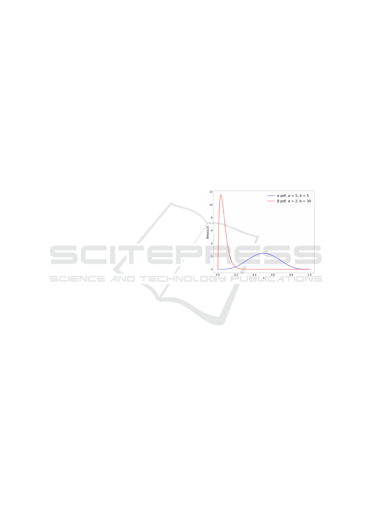
3 BEHAVIOUR OF THE VIRUS

There are two main characteristics that make a virus

lethal: infectivity and death rate. Let us consider a

network represented by an undirected graph. Start-

ing from a random node, the infection spreads across

the network. Since the viral quantity of the virus in

the human body follows an exponential trend over

time as N

= N

+∞

(1 − e

−λt

), it is reasonable to as-

sume that if person i has been infected at time 0, the

probability of infecting each neighbour is deﬁned as:

= α

(1 − e

−λt

) while the probability of his death is

= β

(1−e

−λt

), where both α

and β

are distributed

according to Beta distributions, characterized by dif-

ferent parameters (see Figure 1), and λ is the param-

eter to be optimized in order to maximize the number

of deaths. We can consider the following ﬁve states

for each node:

• Healthy: the person was not infected with the

virus;

• Contagious: the person was infected with the

virus and has a viral quantity different from zero,

therefore she/he can infect other people;

• Ill: as soon as the viral quantity exceeds the

threshold value h, 1 − e

−λt

≥ h, the person be-

comes ill and she/he is removed from the network,

in this way the quarantine period is simulated;

• Recovered: the ill person survived for T times-

tamps, hence she/he is considered healed;

• Dead: the ill person could not recover within the T

timestamps, therefore she/he is considered dead.

Figure 2 shows the ﬂow diagram of the states a

node might go through during the simulation. Consid-

ering implementation issues, the most suitable layer

for supporting the described, ﬂexible behaviour is rep-

resented by an XML data storage layer (e.g., (Can-

nataro et al., 2002b; Bonifati and Cuzzocrea, 2007;

Cannataro et al., 2002a; Cuzzocrea et al., 2009a)).

Figure 1: Beta distributions for both probability p to infect

someone else and probability q to die and the relative pa-

rameters.

4 THE NETWORK GRAPH

The network that has been considered is a 3000 nodes

undirected stochastic block model graph composed

by three communities. The composition of the com-

munities is deﬁned in such a way that the three com-

munities include, respectively, 14%, 50% and 36% of

the total number of nodes. The connections among

nodes in the graph are established according to the

symmetric edge probability matrix P,

P =





0.01 0.001 0.001

0.001 0.005 0.0008

0.001 0.0008 0.005





The elements on the diagonal of matrix P de-

scribe the probability to establish connections be-

tween nodes within the same community, while the

off-diagonal elements describe the probability to con-

nect nodes belonging to different communities. Being

ICEIS 2022 - 24th International Conference on Enterprise Information Systems

188

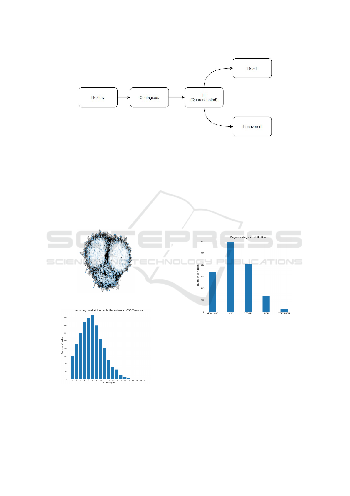
Figure 2: Flow diagram of node’s states.

the probabilities in matrix P quite small, it is likely

that some nodes will be isolated and, since patient

zero is randomly picked at the beginning of the sim-

ulation, in order to let the virus spread carry on, each

node is forced to have at least degree 3. The obtained

network has an average degree of 7.842, an average

node closeness centrality equal to 0.241 and its de-

gree distribution is shown in Figure 4. The graph is

shown in Figure 3 and it is possible to identify the

three distinct communities composing the stochastic

block model graph.

Figure 3: The actual graph of 3000 nodes.

Figure 4: Degree distribution for the stochastic block model

graph of 3000 nodes.

Each node has also been characterized by an addi-

tional information, the degree category, which identi-

ﬁes the connectivity in broad terms of the node itself

towards the other nodes. In order to obtain this infor-

mation, the values of the node degree distribution are

subdivided into ﬁve categories. The ﬁve possible de-

gree categories are: very low, low, medium, high and

very high. By observing the degree category distri-

bution in Figure 5, it becomes clear that the vast ma-

jority of the nodes are characterized by a degree cat-

egory which is either very low, low or medium; very

few are, instead, characterized by a very high degree

category. This additional information is necessary to

observe the behaviour of the virus spread by selecting

a different degree category for the patient zero.

Figure 5: Degree category distribution of the nodes in the

graph.

5 THE SIMULATION

Having deﬁned the graph, the parameters of the nodes

populating the graph are initialized.

More in detail, for a node i, the probability to in-

fect p

and the probability to die q

are set to zero,

since at the beginning of the simulation all the nodes

are assumed to be healthy, and the parameters α

and

, which rule respectively p

and q

, are drawn from

the beta distributions.

The experiment is a discrete-event simulation

which takes as input the graph with its nodes and the

Virus Spread Modeling and Simulation: A Behavioral Parameters Approach and Its Application to Covid-19

189

maximum duration in timestamps. It is also possible

to specify as input the degree category of the patient

zero or to select a speciﬁc node as patient zero. Each

timestamp of the simulation corresponds to 2 days.

5.1 Infection and Illness

In the ﬁrst iteration, the patient zero node is set to be

contagious, which means that for the next iterations it

is able to infect other nodes. In the following itera-

tions, the contagious node i try to infect its neighbors.

To decide whether the neighbor node j is infected or

not by the node i, a random number is extracted from

a uniform distribution and, if it is less than p

, also

node j becomes contagious. Since the probability p

and the viral quantity are time dependent, their val-

ues are updated at each iteration for all the contagious

nodes. Sooner or later, the viral quantity of a conta-

gious node will exceed the threshold h. The occur-

rence of this event causes a state change for the node,

from the contagious state to the ill state and, from now

on, the node is forced to be in quarantine, therefore it

is not able to infect other nodes anymore. As soon as

the node becomes ill, a local counter is initialized and

incremented, iteration by iteration, for the whole ill-

ness period, and its probability to die q is initialized.

For each iteration during which the node is in the ill

state, the value of q is updated, being also its value

time dependent.

5.2 Death

Once the node i is ill, at each new iteration a random

number is drawn from a uniform distribution. If this

random number is smaller than the probability to die,

, the node is considered dead, otherwise it survives

for another iteration.

5.3 Healing

If the node is strong enough to survive the virus for a

number of iterations equal to T, the node is considered

recovered. At this point the node is immune to the

virus, it can not be infected anymore and neither it

can infect other nodes.

5.4 End of the Simulation

The simulation stops as soon as all the nodes within

the network are either healthy, healed or dead. This

scenario corresponds to not having contagious nodes

anymore, the virus spread is stopped and, in the re-

maining iterations, the ill nodes ﬁght for their lives.

6 REAL PARAMETERS

DISCOVERY

The goal of the research is to maximize the mortality

of the virus. Since the virus behaviour is driven by

the parameters h, T and λ, by setting the values of

h and T to extremely high numbers, all the nodes of

the network will eventually die. This would make the

optimization problem trivial.

In order to model a realistic virus, the infectivity

and mortality targets are deﬁned. The ﬁrst one is set to

40%, while the second one to 7%

. The percentages

refer to the total amount of nodes in the network.

Several values for h and T are tested, and the pairs

of values that, jointly, get the closest to the percent-

age targets are considered. The values for λ are taken

in the interval (0,1), excluding the extremes, which

would give contagious and death probabilities that are

either null or quickly converging to α

and β

More in detail, the analyzed values for h, T and λ

are taken from the following ranges:

• h ∈ [0.3, 0.6], with a step of 0.05;

• T ∈ [3, 4, 5, 6];

• λ ∈ [0.05, 0.99], with a step of 0.05.

The discovery of the real (h, T ) parameters has

been carried out by selecting a patient zero node with

a degree category equal to medium. This choice pro-

vides results that are far away from the extreme sce-

narios about having either a very scarce neighborhood

or a very populated one.

For each executed simulation, characterized by a

speciﬁc triplet (h, T, λ), the discrepancy between the

actual percentage of infected nodes and the infectiv-

ity target is computed. Similarly, the discrepancy be-

tween the actual number of deaths and death target

is also discovered. The two discrepancies are then

summed up. Therefore, for each duplet of tested val-

ues (h, T ), an overall distance from the targets is ob-

tained.

Sorting the pairs (h, T ) by ascending order with

respect to the distance from the targets, only those

ones with a distance smaller than 500 are kept. The

real values for (h, T) are discovered by averaging the

obtained values. The whole list of obtained results is

shown in the following table:

The reason behind considering all the pairs (h, T )

with a distance from the targets lower than 500 relies

on the fact that, being the simulation a random exper-

iment, the same triplet (h, T, λ) could provide slightly

Percentages were chosen considering past pandemics,

such as the infections around the world caused by the Span-

ish inﬂuenza and the deaths for syphilis in Europe during

the XV century(Morens et al., 2020).

ICEIS 2022 - 24th International Conference on Enterprise Information Systems

190

Table 1: The (h,T) pairs closest to the chosen target.

h T sum of target differences

0.3 3 17

0.45 3 136

0.4 3 176

0.35 3 229

0.55 5 342

0.45 5 372

0.3 6 374

0.3 3 432

0.5 3 434

0.3 5 446

0.55 3 487

different results over different experiments. Hence,

to alleviate this variability, a larger set of results was

considered.

The obtained real (h, T) parameters, for the net-

work of 3000 nodes, are the following:

• h = 0.45;

• T = 4.

7 LAMBDA OPTIMIZATION

In classical literature, optimization is a critical aspect

to be considered (e.g., (Cuzzocrea, 2005; Cuzzocrea

and Chakravarthy, 2010; Cuzzocrea et al., 2009b;

Cuzzocrea et al., 2003; Ceci et al., 2015)). With sim-

ilar emphasis, here we focus on how to improve sim-

ulation runs.

Now that the real (h, T ) parameters have been dis-

covered, the focus is aimed at λ and its value that

achieves the highest number of deaths in the network.

The analyzed values of λ are taken from the fol-

lowing range:

• λ ∈ [0.2, 0.7], with a step of 0.01.

So now, a more detailed range for λ is consid-

ered. The reason why the range extremes have been

reduced is given by the fact that some values of λ, ei-

ther too high or too small, provide results too far from

the virus targets previously discussed (6).

Running different simulations, the just discovered

real parameters (h, T ) are kept ﬁxed, while λ is let

vary in the mentioned range.

The patient zero, for each simulation, has been

drawn from the list of nodes of the medium degree

category, and the number of executed simulations is

such that 20% of the nodes belonging to it are se-

lected. The reason behind this broad research is to

provide a more reliable assessment on the optimal λ

value, considering the stochastic nature of the simula-

tion.

The λ values that achieved the highest number of

deaths are reported in Figure 6.

The selected value for the optimal lambda corre-

sponds to the most recurrent lambda that achieved the

highest number of deaths. Therefore, λ

opt

= 0.59 is

the selected optimal lambda.

Figure 6: The ﬁve most recurrent lambdas that achieved the

highest number of deaths.

8 FINAL SIMULATION WITH

THE DISCOVERED

PARAMETERS

The triplet of parameters (h, T, λ), that jointly satis-

ﬁes the infectivity and death targets and provides the

most deaths, has been discovered. A ﬁnal single sim-

ulation has been executed to analyze the virus spread

evolution over time and the nodes behaviour. Figure 7

shows the results of the simulation. The patient zero

is randomly selected from the subset of nodes with a

medium degree category.

The simulation lasts 21 iterations, therefore the

virus spread takes 42 days to cease. One third of the

nodes never gets in touch with contagious nodes, and

most of the infected nodes heal from the virus, as ex-

pected. Also the total amount of ill and dead nodes

roughly respects the imposed targets; unfortunately, it

not possible to totally respect the targets, because of

the random nature of the simulation.

It can be also noticed that the temporal evolution

of the virus spread follows the SIR epidemic trend

(Keeling and Danon, 2009), in which, starting with

all the nodes being healthy, the infection begins and

Virus Spread Modeling and Simulation: A Behavioral Parameters Approach and Its Application to Covid-19

191

Figure 7: Network behaviour, patient zero of degree “MEDIUM”.

the number of ill nodes starts increasing. Once the

peak of ill nodes reaches its maximum, both recov-

ered and dead nodes increase, until a stable situation

is reached.

In order to further exploit and extend the described

simulation model, network-based solutions would be

necessary (e.g., (Cuzzocrea et al., 2005; Cuzzocrea

et al., 2004; Bellatreche et al., 2010)).

9 CONCLUSIONS AND FUTURE

WORK

The analysis carried out in this report shows that it is

possible to model a realistic virus’ behaviour, that sat-

isﬁes both illness and death targets, by properly tun-

ing the modelling parameters.

Furthermore, it has been shown that the network

characteristics play a fundamental role on the out-

come of the experiment. It is fair to state that, as the

overall connectivity of network increases, the virus

spreads more efﬁciently in the network, which might

be intuitive.

It has been also proved that the degree of the pa-

tient zero has a great impact on the development of

the virus spread, which conﬁrms that a prompt con-

tainment of the virus is extremely effective to reduce

the virus spread, especially if the virus outbreak starts

in less connected portions of the network.

Obviously, the characteristics of the virus play a

major role. It has been discovered that the best set-

ting allows the virus to quickly spread and have a high

probability to kill the ill nodes, but not high enough

to cause the immediate death of the contagious nodes,

which would result in the death of the virus itself.

This means that, in a real case scenario, it would not

be sufﬁcient for the health system to monitor only dis-

eases causing severe symptoms.

Finally, it may be said that the employed virus

model is quite simplistic, described by few parame-

ters, but it shows a glance of a general behaviour for

the spread of a virus, similar to the more sophisticated

SIR model.

Future work is mainly oriented to apply the de-

scribed simulation framework to innovative big data

applications (e.g., (Braun et al., 2017; Audu et al.,

2019; Ahn et al., 2019; Morris et al., 2018)).

ACKNOWLEDGEMENTS

This research has been partially supported by

the French PIA project “Lorraine Universit

d’Excellence”, reference ANR-15-IDEX-04-LUE.

The authors are grateful to R. Gallo, M. Baiocchi,

P. Migneco, M. Sangiorgio for their contribution.

REFERENCES

Ahn, S., Couture, S. V., Cuzzocrea, A., Dam, K., Grasso,

G. M., Leung, C. K., McCormick, K. L., and Wodi,

B. H. (2019). A fuzzy logic based machine learning

tool for supporting big data business analytics in com-

plex artiﬁcial intelligence environments. In FUZZ-

IEEE 2019, New Orleans, LA, USA, June 23-26, 2019,

pages 1–6. IEEE.

Alassaﬁ, M. O., Jarrah, M., and Alotaibi, R. (2022). Time

series predicting of COVID-19 based on deep learn-

ing. Neurocomputing, 468:335–344.

Audu, A. A., Cuzzocrea, A., Leung, C. K., MacLeod, K. A.,

Ohin, N. I., and Pulgar-Vidal, N. C. (2019). An in-

telligent predictive analytics system for transportation

analytics on open data towards the development of a

smart city. In CISIS 2019, Sydney, NSW, Australia, 3-5

July 2019, pages 224–236. Springer.

ICEIS 2022 - 24th International Conference on Enterprise Information Systems

192

Bellatreche, L., Cuzzocrea, A., and Benkrid, S. (2010).

F&A: A methodology for effectively and efﬁciently

designing parallel relational data warehouses on het-

erogenous database clusters. In DAWAK 2010, Bil-

bao, Spain, August/September 2010, pages 89–104.

Springer.

Bonifati, A. and Cuzzocrea, A. (2007). Efﬁcient fragmen-

tation of large XML documents. In DEXA 2007, Re-

gensburg, Germany, September 3-7, 2007, pages 539–

550. Springer.

Braun, P., Cuzzocrea, A., Keding, T. D., Leung, C. K., Paz-

dor, A. G. M., and Sayson, D. (2017). Game data

mining: Clustering and visualization of online game

data in cyber-physical worlds. In KES 2017, Mar-

seille, France, 6-8 September 2017, pages 2259–2268.

Elsevier.

Cannataro, M., Cuzzocrea, A., Mastroianni, C., Ortale, R.,

and Pugliese, A. (2002a). Modeling adaptive hyper-

media with an object-oriented approach and XML. In

WebDyn@WWW 2002, Honululu, HW, USA, May 7,

2002, pages 35–44. CEUR-WS.org.

Cannataro, M., Cuzzocrea, A., and Pugliese, A. (2002b).

XAHM: an adaptive hypermedia model based on

XML. In SEKE 2002, Ischia, Italy, July 15-19, 2002,

pages 627–634. ACM.

Ceci, M., Cuzzocrea, A., and Malerba, D. (2015). Ef-

fectively and efﬁciently supporting roll-up and drill-

down OLAP operations over continuous dimensions

via hierarchical clustering. J. Intell. Inf. Syst.,

44(3):309–333.

Cuzzocrea, A. (2005). Overcoming limitations of approx-

imate query answering in OLAP. In IDEAS 2005,

25-27 July 2005, Montreal, Canada, pages 200–209.

IEEE Computer Society.

Cuzzocrea, A. and Chakravarthy, S. (2010). Event-based

lossy compression for effective and efﬁcient OLAP

over data streams. Data Knowl. Eng., 69(7):678–708.

Cuzzocrea, A., Darmont, J., and Mahboubi, H. (2009a).

Fragmenting very large XML data warehouses via k-

means clustering algorithm. Int. J. Bus. Intell. Data

Min., 4(3/4):301–328.

Cuzzocrea, A., Furfaro, F., Greco, S., Masciari, E., Mazzeo,

G. M., and Sacc

a, D. (2005). A distributed system

for answering range queries on sensor network data.

In PerCom 2005 Workshops, 8-12 March 2005, Kauai

Island, HI, USA, pages 369–373. IEEE Computer So-

ciety.

Cuzzocrea, A., Furfaro, F., Masciari, E., Sacc

a, D., and Sir-

angelo, C. (2004). Approximate query answering on

sensor network data streams. GeoSensor Networks,

49.

Cuzzocrea, A., Furfaro, F., and Sacc

a, D. (2003). Hand-

olap: A system for delivering OLAP services on hand-

held devices. In ISADS 2003, 9-11 April 2003, Pisa,

Italy, pages 80–87. IEEE Computer Society.

Cuzzocrea, A., Furfaro, F., and Sacc

a, D. (2009b). En-

abling OLAP in mobile environments via intelligent

data cube compression techniques. J. Intell. Inf. Syst.,

33(2):95–143.

Dodds, W. (2019). Disease now and potential future pan-

demics. The World’s Worst Problems, page 31–44.

Godio, A., Pace, F., and Vergnano, A. (2020). Seir model-

ing of the italian epidemic of sars-cov-2 using compu-

tational swarm intelligence. IJERPH, 17.

Harckbart, G. (2020). Heterogeneous siqr models with mass

testing and targeted quarantine and the spread of in-

fectious disease.

Hasaninasab, M. and Khansari, M. (2022). Efﬁcient

COVID-19 testing via contextual model based com-

pressive sensing. Pattern Recognit., 122:108253.

Keeling, M. J. and Danon, L. (2009). Mathematical mod-

elling of infectious diseases. British Medical Bulletin,

92(1):33–42.

Kurtin, D. L., A.J., D., and Stagg, S. M. (2020). VTES:

a stochastic python-based tool to simulate viral trans-

mission [version 1]. F1000Research.

Li, S. and Yan, Y. (2022). Data-driven shock impact of

COVID-19 on the market ﬁnancial system. Inf. Pro-

cess. Manag., 59(1):102768.

Mishra, B. K. and Singh, A. K. (2011). Two quarantine

models on the attack of malicious objects in computer

network. Hindawi Publishing Corporation.

Morens, D. M., Daszak, P., Markel, H., and Taubenberger,

J. K. (2020). Pandemic covid-19 joins history’s pan-

demic legion. mBio, 3(11).

Morris, K. J., Egan, S. D., Linsangan, J. L., Leung, C. K.,

Cuzzocrea, A., and Hoi, C. S. H. (2018). Token-based

adaptive time-series prediction by ensembling linear

and non-linear estimators: A machine learning ap-

proach for predictive analytics on big stock data. In

ICMLA 2018, Orlando, FL, USA, December 17-20,

2018, pages 1486–1491. IEEE.

Ronaghi, F., Salimibeni, M., Naderkhani, F., and Mo-

hammadi, A. (2022). COVID19-HPSMP: COVID-19

adopted hybrid and parallel deep information fusion

framework for stock price movement prediction. Ex-

pert Syst. Appl., 187:115879.

Yadav, A. and Vishwakarma, D. K. (2022). A language-

independent network to analyze the impact of

COVID-19 on the world via sentiment analysis. ACM

Trans. Internet Techn., 22(1):28:1–28:30.

Virus Spread Modeling and Simulation: A Behavioral Parameters Approach and Its Application to Covid-19

193