
Opti-Soft+: A Recommender and Sensitivity Analysis for Optimal
Software Feature Selection and Release Planning
Fernando Boccanera and Alexander Brodsky
Computer Science Department, George Mason University, Virginia, U.S.A.
Keywords: Decision Guidance System, Decision Support System, Software Release Planning, Optimization, Mixed-
Integer Linear Programming.
Abstract: Many approaches have been developed to increase the return on a software investment, but each one has
drawbacks. Proposed in this paper is the Opti-Soft+ framework that addresses this problem by producing a
software release schedule that maximizes the business value of investments in information systems that
automate business processes. The optimal release schedule is the result of solving a mixed integer linear
programming problem. Opti-Soft+ is an extension of the Opti-Soft framework proposed earlier with (1) a
refined cost model, (2) a technique for sensitivity analysis of the normalized cost per unit of production, and
(3) an atomic business process model that is driven by output throughputs in addition to input throughputs.
1 INTRODUCTION
Software development projects that are successful
and return to the business a value that justify their
investments are not common. According to (The
Standish Group, 2018) only 36% of projects are
successful. To improve the rate of success,
organizations have been using Agile methods. As
reported in (Serrador & Pinto, 2015,) Agile does have
a statistically significant impact on three dimensions
of project success, but adopting Agile is not a
guarantee of a return on the investment.
Because the Agile software development
lifecycle is based on short iterations, at each iteration
the team needs to decide what functionality to
include. This process, called Release Planning,
provides an opportunity to improve the business value
of the software because different functionalities result
in different value profiles.
Several release planning approaches have been
developed to maximize the business value of software
delivery. The highly influential Incremental Funding
Methodology (IFM) by (M. Denne & Cleland-Huang,
2004) uses heuristics to select a release schedule that
maximizes the business value of software
investments. F-EVOLVE*’s approach (Maurice et
al., 2006) is to involve stakeholders iteratively to
achieve releases that result in the highest degree of
satisfaction. A third approach by (Van den Akker et
al., 2005) applies integer linear programming to
maximize the revenue.
The IFM, F-EVOLVE* and Van den Akker
approaches use cash flow as a proxy for business
value. They all require the estimation of cash flows
for each software feature and that’s very challenging
due to the difficulty of drawing a direct correlation
between a particular business benefit, like a reduction
in cost, and a specific piece of software. (Devaraj &
Kohli, 2002) have acknowledged this difficulty of
isolating the effect of IT on firm performance.
The main pitfall of the existing approaches is
imprecision. Also, every dollar of cash flow needs to
be allocated to one and only one feature which is not
a realistic assumption, because often, realizing a
business benefit requires the implementation of
multiple software features. Another pitfall is that each
cash flow estimate combines the business benefit with
the software development cost, which means that all
the estimations have to be done externally, which is
typically difficult and often inaccurate.
In (Boccanera & Brodsky, 2020) and (Boccanera
& Brodsky, 2021), we proposed a new approach,
called Opti-Soft, to address the pitfalls of existing
methods for a class of software projects that automate
a Business Process Network (BPN). Opti-Soft is a
decision guidance framework for release planning
that maximizes the business value as measured by the
Net Present Value (NPV), based on a model of the
underlying business process and savings achieved
500
Boccanera, F. and Brodsky, A.
Opti-Soft+: A Recommender and Sensitivity Analysis for Optimal Software Feature Selection and Release Planning.
DOI: 10.5220/0011062400003179
In Proceedings of the 24th International Conference on Enterprise Information Systems (ICEIS 2022) - Volume 1, pages 500-513
ISBN: 978-989-758-569-2; ISSN: 2184-4992
Copyright
c
2022 by SCITEPRESS – Science and Technology Publications, Lda. All rights reserved

due to the combined effect of new software features
on improved business process efficiency.
However, the Opti-Soft approach has limitations,
as we discovered looking at a number of real software
project examples. First, the cost model was based on
labor costs only, whereas realistic cost models may be
considerably more involved. Second, for stakeholders
to have a high confidence on the recommendations on
software feature selection and release planning, they
often need to know the sensitivity of the
recommendations to assumptions on demand on
business process throughput, e.g., the number of daily
patent applications to be processed by the Patent
Office. Third, while the business processes can be
hierarchically composed, Opti-Soft only supported a
limited atomic (leaf) process in the hierarchy in which
the cost is driven by input throughput (e.g., number of
patent applications that need to be processed per day).
Whereas, atomic processes driven by output
throughput were not supported.
Lifting these limitations is exactly the focus of
this paper. More specifically, the contributions of this
paper are as follows. First, we extend the cost model,
of both BPN and software development, beyond labor
cost to include a range of variable and fixed costs (i.e.,
of resources required).
Second, we develop a technique for sensitivity
analysis of the normalized cost per unit of production,
for a recommended release plan and associated
improved BPN, as a function of BPN throughput. The
analysis involves fixing some of the decision
variables while allowing others to be instantiated by
the optimizer. The idea is to determine the delta
change in the objective function for a one-unit change
of the required BPN throughput.
Third, we develop an atomic service model that is
driven by output throughputs in addition to the one
driven input throughputs.
Opti-Soft+ is the result of these extensions. It
takes advantage of the fact that the implementation of
software features leads to more efficient business
processes due to a reduction of the time a worker
spends, or the elimination of a portion of the process,
or the utilization of workers with a lower labor rate.
The key idea is that, because the improved business
efficiency is a direct consequence of the availability
of software features, this relationship can be formally
modelled using mixed integer linear programming
(MILP) constraint formulation, which allows the use
of MILP solvers to find optimal release plan.
The uniqueness of Opti-Soft+ framework is its
accurate estimate of business value improvement by
formally modeling BPN and associated costs over the
investment time horizon, as a function of chosen
software features and release plan. Also, Opti-Soft+
removes the limitation of existing approaches that
force every investment dollar to be assigned to one
and only one software feature. The Opti-Soft+ model
allows one software feature to impact multiple
processes and allows a process to be impacted by
multiple features, on a many-to-many relationship. In
Opti-Soft+, the estimation of the business value of
software features is not external to the approach, but
instead, is at the heart of the cost model. The Opti-
Soft+ framework is composed of a methodology, a
formal optimization model and a Decision Guidance
System (DGS) which implements the formal model
and produces an optimal recommendation.
This paper is organized as follows: Section 2
provides an overview of the Opti-Soft+ model,
including the cost approach, the BSN modeling and
release planning. Section 3 briefly describes the
optimization model; Section 4 describes the DGS and
the methodology; Section 5 provides an example of
the extensions; Section 6 conducts a sensitivity
analysis and Section 7 provides concluding remarks.
Appendix 1 shows the entirety of the formal model.
2 OPTI-SOFT+ MODEL
OVERVIEW
In order to maximize the business value associated
with new software features, we need to estimate the
cost of software development as well as the benefit of
the implementation of the software. For software that
implements information systems to automate a
business process, the benefit of the software is the
cost savings in the business process due to
automation.
A business process consumes input flows and
produces output flows. The cost associated with the
business process is a function of the cost drivers such
as labor rates and time spent. This means that the
benefit (savings) of a software feature that automates
a business process can be determined by subtracting
the cost of the automated process from the cost of the
process before automation.
The above insight, that the implementation of
software features allows the adoption of more
efficient business process networks (BPN) is key to
Opti-Soft+, because each new BPN configuration can
be modelled, and its cost measured. In the Opti-Soft+
approach, there is no need to estimate the cost of each
individual feature, a feature is just a device that
triggers a change in the BPN configuration, while cost
is precisely calculated at the level of the BPN.
Opti-Soft+: A Recommender and Sensitivity Analysis for Optimal Software Feature Selection and Release Planning
501
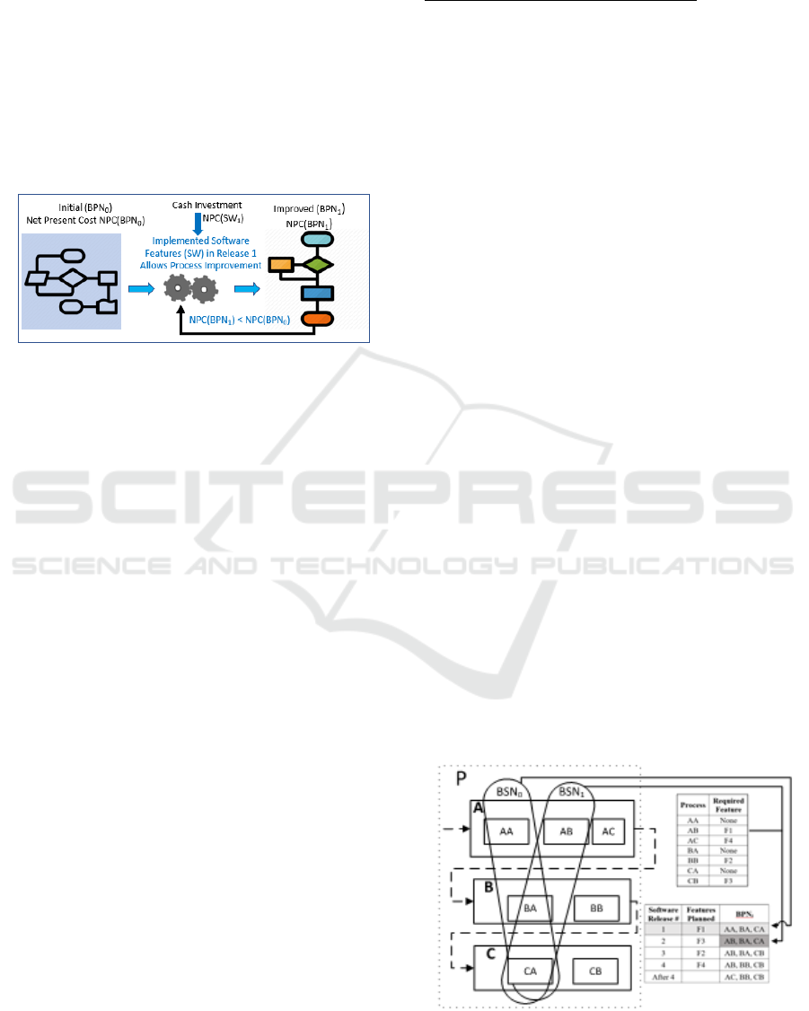
In Figure 1, we have an initial BPN configuration,
called BPN
0
that can benefit from automation and has
a Net Present Cost NPC(BPN
0
). A cash investment,
NPC(SW
1
) is made to implement software features
SW
1
in the first release (r=1). After release 1, the
availability of the software features SW
1
allow
process improvements so BPN
0
transitions to BPN
1
,
resulting in a Net Present Cost NPC(BPN
1
), which is
lower than NPC(BPN
0
). The procedure continues
iteratively, with each investment NPC(SW
r
) in
release r, causing the BPN
r-1
to transition to BPN
r
,
resulting in a lower NPC(BPN
r
).
Figure 1: BPN Cost Reduction due to the Investment in
Software Features.
In order to calculate and optimize the cost savings,
we need to model the BPN transitions as well as the
enabling software development features.
BPN Modeling
To intuitively understand BPN modeling, consider
the example depicted in Figure 2. It shows a parent
process P composed of subprocesses A, B and C, all
of which must be executed. Note that the output from
A serves as input to B and the output from B serves
as input to A. Subprocess A has three alternatives,
AA, AB and AC, whereas only one of them must be
executed. Similarly, B has alternatives BA and BB,
and C has alternatives CA and CB. By choosing
among the alternatives for each subprocess, a new
configuration of P is established.
Note that a valid configuration for P requires one
and only one of each of its three subprocesses A, B
and C, which establishes an AND relationship
between process P and its subprocesses A, B and C.
The relationship between A and its alternatives
(subprocesses) AA, AB and AC is an OR because
either AA or AB or AC can be present in P. B and C
also have OR relationships with their subprocesses.
We model the BPN as a Service Network (SN)
(Brodsky et al., 2017) which is a “network of service-
oriented components that are linked together to
produce products”. We use the term Business Service
Network (BSN) to refer to the BPN as a SN. The
linkage among service components is through inputs
and outputs. In Figure 2, P is a composite (parent)
service because it is composed of subservices A, B
and C. A, B and C are also composites while all the
other subservices are atomic, that is, indivisible.
BSN Transition and Release Planning
The transition from a subprocess alternative to
another requires the implementation of specific
software functionality called features. For example,
subprocess alternative AB requires feature F1.
We assume that features are implemented in
iterations called releases. At the beginning of each
release, the team decides which features to include in
the scope. This is called release planning. Note that
the implementation of features results in automation
of certain aspects of the original business process,
allowing it to transition to a more efficient process
alternative that results in labor and other savings.
In the example of Figure 2, we assume that AA,
BA and CA are manual processes, and the initial BPN
configuration (BPN
0
) is AA, BA, CA with
NPC(BPN
0
). The top table on the right shows the
required features for each process while the table on
the bottom shows the BPN configuration after each
release. Note that A’s alternative subprocess AB is
more cost effective than AA and it requires feature
F1. Because F1 is implemented in release 1, after
release 1 is completed, BPN
0
transitions to BPN
1
which is configured with AB, BA, CA, with the cost
of NPC(BPN
1
).
Note that F1 ‘activates’ AB and this
activation property, which is unique to Opti-Soft+, is
used extensively in the formalization of the Mixed
Integer Linear Programming problem, described in
section 3. At the end of each release, the availability
of implemented software features allows the
activation of alternative processes that are more cost
effective, reducing the overall NPC of the SN.
Subprocess AA transitions to AB then to AC, BA
transitions to BB and CA transitions to CB. The final,
optimal SN configuration is then AC, BB, CB. Note
that Fig 2 shows not only the BSN transitions, but also
the release plan, that is, the software features
implemented in each release.
Figure 2: Example of BPN Transition as a result of feature
delivery.
ICEIS 2022 - 24th International Conference on Enterprise Information Systems
502

Cost Model
The NPC over the investment time horizon is the
combined NPC of all the BPNs plus the NPC of
software development in all releases. Costs are
accrued daily and are paid on a set schedule. The NPC
is composed of five types of cost:
1. Variable labor costs of the SN
2. Variable non-labor costs of the SN
3. Fixed non-labor costs of the SN
4. Variable labor costs of software features
5. Fixed non-labor costs of software features
Note that in the Opti-Soft+ model, we use the Net
Present Value (NPV), which is simply NPC with the
negative sign.
Variable Labor Costs of the SN
Each process of the SN is performed by workers with
well-defined roles. Each role has a labor rate and each
input processed or output produced by the role has a
set duration. The cost of a process, or
LaborCostPerDay, is the labor rate times the duration
to handle all inputs and outputs in a day.
Variable Non-labor Costs of the SN
Variable, non-labor costs are associated with the
amount of work produced by an atomic service, that
is, is driven by the inputs or by outputs and are
similar to the calculation of labor costs.
Parameters CostPerInput and CostPerOutput
capture the non-labor costs for each input and output.
These parameters are used to compute
FlowCostPerDay.
Fixed Non-labor Costs of the SN
Fixed non-labor costs are not driven by inputs or
outputs, instead they are driven by the services. An
example of a fixed cost associated with a particular
service is rent. Parameter ServiceCostPerDay
captures the daily cost for each atomic service and is
used to calculate the ServiceCostPerDay.
Variable Labor Costs of Software Development
Opti-Soft+ follows an Agile practice called feature-
driven, where release planning is done at the feature
level, that is, features are removed from the product
backlog and assigned to releases. The size of features
is estimated in points, which is a unit based on the
perceived effort to develop the feature. The release
size, that is, the sum of the points for all features in
the release, cannot exceed the capacity of the team,
which is the average productivity of a developer times
the size of the team. Development labor cost, in turn,
is computed by multiplying the team’s capacity by the
developer cost per effort point. The formal model
captures the software cost in SWCostPerDay and then
uses a pay schedule to calculate the LaborCashFlow.
Fixed Non-labor Costs of Software Development
Fixed costs associated with features are experienced
during software development, where features are
produced. They are incurred by resources such as a
hardware server, a software tool, etc…
Every feature requires a set of resources. The full
set of resources required by a feature f needs to be
available prior to the start of the release that
implements f. A resource might be paid in the release
that implements f or in a prior release. We assume that
resource costs are paid on the first day of each release,
consequently on the first day of a release, all
resources needed by all features in the release must be
paid.
To be flexible, we allow multiple features to
require the same resource, establishing dependencies
among features. Resource dependencies are handled
by a Dependency Graph.
The cost of resources is captured in ResCashFlow,
whose computation uses the following parameters:
𝑹𝒆𝒔𝑺𝒆𝒕 is the set of all non-labor resources
𝑭𝒆𝒂𝒕𝒖𝒓𝒆𝑹𝒆𝒔 maps features to resources
𝑹𝒆𝒔𝑪𝒐𝒔𝒕 maps a resource to its cost
Computation of the SN Cash Flow
The CostPerDay of each atomic process is the sum of
LaborCostPerDay, FlowCostPerDay and
ServiceCostPerDay. CostPerDay is used to calculate
the schedule of payments, or CashFlow(d) for each d
in the time horizon. The CashFlow(d) for each
subprocess of a parent process is aggregated and then
rolled up to determine the CashFlow(d) of the entire
SN.
Computation of the Software Cash Flow
The CashFlow(d) of the development of software is
the sum of LaborCashFlow and ResCashFlow.
Computation of NPV
The CashFlow(d) for the SN and for the Software
Development are combined and discounted to
produce the TimeWindowNPV.
3 OPTI-SOFT+ OPTIMIZATION
MODEL
Opti-Soft+ produces an optimal release schedule and
SN configuration by solving a maximization problem
given a set of parameters like the services in the SN,
feature sizes, number of releases, time horizon, labor
rates, size of the development team, etc... It
maximizes the NPV of the total cost of the service
network plus the software development cost over the
investment horizon, subject to constraints such as the
Opti-Soft+: A Recommender and Sensitivity Analysis for Optimal Software Feature Selection and Release Planning
503

space of process alternatives. Opti-Soft+’s formal
model with its parameters, computations, constraints
and maximization formulation is presented in its
entirety in Appendix 1.
The formulation of the optimization is of a Mixed-
Integer Linear Programming (MILP) problem,
because 1) three of the DVs (On(s,r), IBF(r,f),
ITF(r,f)) are Boolean, 2) one DV (InputThru(s,i,r)) is
real, and 3) the objective function is linear because it
is the result of the addition of various cost parameters
which themselves are linear. Section A9 of Appendix
1 describes the MIPL formulation, which is
summarized below:
𝑮𝒊𝒗𝒆𝒏 𝑷𝒂𝒓𝒂𝒎𝒆𝒕𝒆𝒓𝒔
𝑴𝒂𝒙 𝑹𝒆𝒍𝒆𝒂𝒔𝒆𝑺𝒄𝒉𝒆𝒅𝒖𝒍𝒊𝒏𝒈.𝑻𝒊𝒎𝒆𝑾𝒊𝒏𝒅𝒐𝒘𝑵𝑷𝑽
𝒔.𝒕. 𝑹𝒆𝒍𝒆𝒂𝒔𝒆𝑺𝒄𝒉𝒆𝒅𝒖𝒍𝒊𝒏𝒈.𝑪𝒐𝒏𝒔𝒕𝒓𝒂𝒊𝒏𝒕𝒔
The constraints are the space of SN alternative
configurations, the required software features, the
capacity of the development team, etc… Each of the
six formal components shown in Appendix 1
implements constraints that are then aggregated under
ReleaseScheduling.Constraints.
Note that the CashFlow and TimeWindowNPV
produced by the formal model are negative numbers
consequently maximizing the NPV results in
minimizing the cost.
4 OPTI-SOFT+ METHODOLOGY
AND DECISION GUIDANCE
SYSTEM
Opti-Soft+ includes a Decision Guidance System
which implements the formal model in Appendix 1
and includes a MILP Solver. It produces:
1. Optimal NPV of the business benefit
2. A release schedule, which is the result of the
Solver instantiating DVs IBF(r,f) and ITF(r,f).
3. The optimal service network configuration at the
end of each release, which is the result of the
Solver instantiating DV On(s,r).
The DGS uses the Parameters in the input file to
maximize the NPV, subject to the Constraints.
During the maximization, the DGS performs the
Computation and chooses the optimal
DecisionVariables. The Opti-Soft+ DGS is
implemented using Unity (Nachawati, M. O.,
Brodsky, A., & Luo, J., 2016), (Nachawati, M. O.,
Brodsky, A., & Luo, J., 2017), a platform for building
DGSs from reusable Analytical Models (AMs). Unity
exposes an algebra of operators and provides an
unified, high-level language called Decision
Guidance Analytics Language (DGAL) (Brodsky,
Alexander, & Luo, J., 2015).
The Opti-Soft+ framework is composed of the
optimization model, the DGS and a methodology. We
covered the first two so now we cover the latter. The
Opti-Soft+ methodology, which extends the
methodology in (Boccanera & Brodsky, 2021),
contains the following steps:
1. Generate candidate software features to be
implemented
2. Capture the As-Is BPN configuration, and
alternative BPN configurations that can be
enabled by candidate software features
3. Gather and instantiate input parameters for the
optimization model as described in Appendix
4. Compute the baseline NPV for the As-Is BPN
5. Perform Opti-Soft+ DGS optimization to come
up with a recommended Release Plan and the
associated optimal BPN configuration (To-Be)
6. Calculate the savings, which is the NPV of the
To-Be minus the NPV of the As-Is
7. During Release 1:
a. Operate the BPN according to the optimal
BPN configuration.
b. Implement recommended software features
8. For each release r = 2,…,n
a. Update existing software features to include
those implemented in the previous release
b. For updated software features and refined
demand/throughput requirements, run
operational optimization to find the best
BPN configuration. Operate the BPN
according to it.
c. Repeat steps above to update the
recommended Release Plan for the
remaining releases (starting from r + 1)
d. Implement recommended software features
5 OPTI-SOFT+ PRODUCES
EXAMPLE OF EXTENSIONS
Sections 5 of (Boccanera & Brodsky, 2021) describe
an example of a service network composed of 3
parent processes (A, B and C). The optimal release
plan and SN configuration, is reproduced in Table 1.
The example has 4 releases, each lasting 60 days and
a time horizon of 520 days, and a BSN that requires
processing 100 user applications per day, that is, for
demand=100. In the example, the optimized objective
function, or NPV, produced by the DGS is
-$6,411,432.73.
ICEIS 2022 - 24th International Conference on Enterprise Information Systems
504
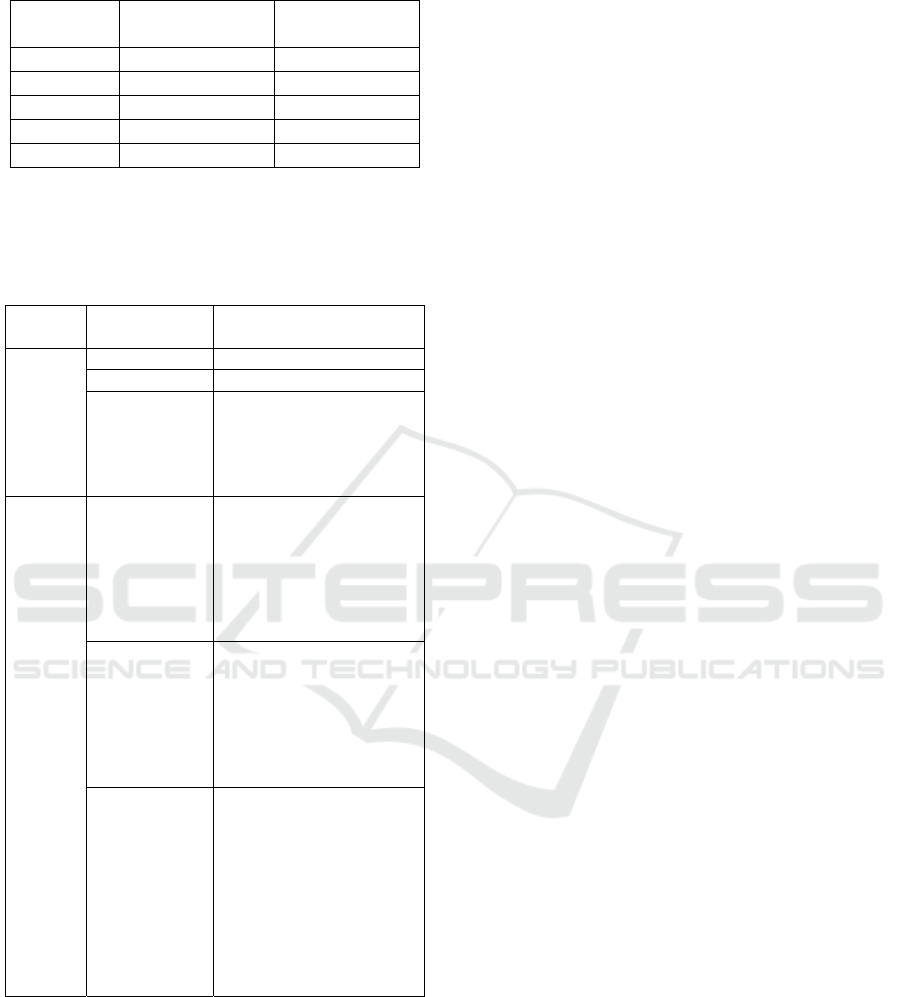
Table 1: Optimal release schedule and SN configuration.
Software
Release #
Features
implemented
Optimal SN
Configuration
1 TF1, BF1 AA, BA, CA
2 BF3 AB, BA, CA
3 BF2 AB, BA, CB
4 BF4 AB, BB, CB
After 4 AC, BB, CB
We now take the example from (Boccanera &
Brodsky, 2021) and add the extensions described in
section 1. Table 2 shows the extended parameters.
Table 2: Extended Parameters.
Forma-
lization
Parameter Value
RSch
R
esSet “softwareLicense1”
R
esCost "softwareLicense1":20,000
F
eatureRes TF1:””
BF1:””
BF2:””
BF3:””
BF4: “softwareLicense1”
I
nput
D
riven
A
tomic
Service
ServiceCost
P
erDay
AA:200
AB:200
AC:200
BA:200
BB:200
CA:200
CB:200
CostPerInput AA.UserApplication:2
AB.UserApplication:0
AC.UserApplication:0
BA.CompliantApplic:0
BB.CompliantApplic:0
CA.AdjudicatedApplic:0
CB.Ad
j
udicatedA
pp
lic:0
CostPerOutput AA.CompliantApplic:3
AA.NonComplianceNtc:1
AB.CompliantApplic:0
AB.NonComplianceNtc:0
AC.CompliantApplic:0
AC.NonComplianceNtc:0
BA.AdjudicatedApplic:0
BB.AdjudicatedApplic:0
CA.AdjudApplicLetter:0
CB.Ad
j
udA
pp
licLetter:0
There is a software license that costs $20,000
when feature BF4 is implemented. There are fixed
costs per day of $200 for each of the atomic processes
(AA, AB, AC, BA, BB, CA, CB). Atomic process AA
incurs $2 in cost per “User Application” input, $3 per
‘CompliantApplication” output and $1 per
“NonCompliantNotice” output.
Using the parameters in Table 2, plus the
parameters in Section 5 of (Boccanera & Brodsky,
2021), the DGS maximizes the objective function and
produces an optimal NPV of -$6,748,777.45. The
increase from -$6,411,432.73 is expected and is a
direct result of the extended costs listed in Table 2.
In order to determine the savings of DGS’
recommendation, we need to compare the NPV of the
extended example (-$6,748,777.45), called the To-
Be, with the NPV of the As-Is, which is the BPN prior
to the development of the software.
To calculate the As-Is recommendation, we
change the example parameters as follows: 1) set to
zero the parameters used in the Software
Development Formal Model and 2) Set the BPN
configuration to AA, BA, CA for the entire duration
of the time horizon of the investment. Running the
DGS with these modified parameters, the resulting
NPV for the As-Is is -$9,611,947.49.
The savings is the difference between the To-Be
(-$6,748,777.45) and the As-Is (-$9,611,947.49), or
$2,863,170.04. Note that this is the maximum
savings, i.e., there is no other release plan and BSN
configuration that produces a higher savings.
6 OPTI-SOFT+ SENSITIVITY
ANALYSIS
One aspect that a decision-maker would be interested
in, is how sensitive the total NPC is to certain changes
in parameters. To answer this, we developed a
technique for sensitivity analysis as follows.
The objective function is the NPV of the cash
outflow of the service network (SN) plus the cash
outflow of developing the software features that allow
the SN to transition to more efficient processes. Opti-
Soft+ has several parameters that influence the NPV,
but the one with the most impact is the demand, which
is the required throughput of the SN. In our example,
the required demand is 100 applications per day.
The required demand, used as a parameter in the
DGS, is an estimation and if there is a high degree of
uncertainty in the estimation, a decision maker might
not have a lot of confidence in the recommendation.
A sensitivity analysis based on the demand parameter
is valuable because it helps to understand risk.
In our sensitivity analysis technique, we use the
NPC instead of the NPV because it is more intuitive.
The goal is to determine the NPC delta, that is, the
additional cost for an increase of one unit of demand.
Given d
0
, the original demand through the SN, we
vary d, the new demand by 1. The delta of the demand
is δ=d-d
0
. We then calculate UC, the cost per unit of
demand d as follows:
Opti-Soft+: A Recommender and Sensitivity Analysis for Optimal Software Feature Selection and Release Planning
505
𝑈𝐶𝛿
𝑁𝑃𝐶𝑑
𝛿
𝑑
𝛿
We can utilize the above technique to conduct two
analyses for a range of δ: 1) fix the release plan and
the BSN configuration, and 2) fix the release plan,
allowing the BSN configuration to be optimized. The
first analysis will show how the unit cost varies with
for each δ, while the second will show the unit cost
variation and the stability of the BSN configuration.
Sensitivity Analysis 1
The steps to conduct analysis number 1 are as
follows: 1) determine a range of δ, above and below
d
0
, to conduct the analysis, 2) run the DGS
optimization with demand=d
0
to get a
recommendation and the value of NPV
0
, 3) instantiate
the ITF(r,f), IBF(r,f) and On(s,r) decision variables
with the release planning schedule and SN
configuration recommended by the DGS in the
previous step, leaving InputThru(s,i,r) as a DV, 4) set
the demand parameter to d
0
+δ
1
, where δ
1
, is the first
value in the δ range, and run the DGS to get the value
for NPC
1
, 5) repeat steps 2-4 (i.e., now performing
operational optimization when software features
available are fixed) for all δ
i
in the range, i >1, 6)
calculate the values of UC(δ
i
), and 7) plot a chart with
the values of δ
i
and UC(δ
i
).
We now apply our sensitivity analysis technique to
the example in Section 4. In step 1, we determine that
the estimated demand d
0
=100 has an error or 10%, so
we set the range of δ to -10 to +10. In step 2 we run
the DGS with demand=100 and produce the
recommendation and NPC
0
=$6,748,777.45,
described in Section 4. In step 3 we instantiate the
release planning schedule and SN configuration DVs
with the recommendation in Section 4. In step 4, we
take the first value in the δ range (-10) and set
demand=100-10=90 and run the DGS, getting
NPC
1
=$6,236,485.38. In step 5, we repeat steps 2-4
for all the other values in the δ range and produce the
NPC results in Table 3. In step 6, we calculate
UC(δ
i
), also shown in Table 3. In step 6 we plot the
chart shown in Fig 3.
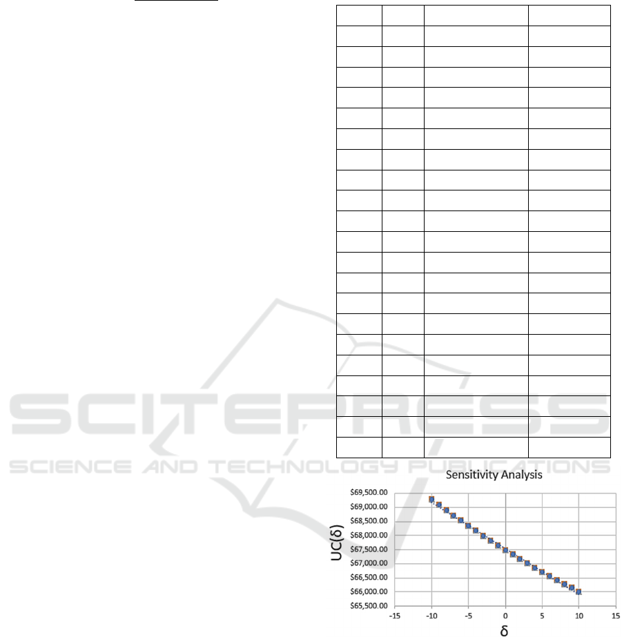
The table and the chart show that as the demand d
increases, the UC, which is NPC per unit of d,
decreases. For a decision maker, this is a desirable
behavior because the initial demand d
0
is just an
estimation. If d
0
was underestimated, then the optimal
NPC is even better than the value provided by the
original recommendation. If d
0
was underestimated, it
is easy to determine the reduction in NPC. This would
help a decision maker to manage the estimation risk
of the demand and consequently yield a higher degree
of confidence in the DGS recommendation.
Table 3: Results of the Sensitivity Analysis.
d δ
NPC(d
0
+ δ)
UC(δ)
90 -10 $6,236,485.38 $69,294.28
91 -9 $6,287,714.60 $69,095.76
92 -8 $6,338,943.82 $68,901.56
93 -7 $6,390,173.05 $68,711.54
94 -6 $6,441,402.27 $68,525.56
95 -5 $6,492,631.49 $68,343.49
96 -4 $6,543,860.71 $68,165.22
97 -3 $6,595,089.93 $67,990.62
98 -2 $6,646,319.15 $67,819.58
99 -1 $6,697,548.37 $67,652.00
100 0 $6,748,777.45 $67,487.77
101 1 $6,800,006.67 $67,326.80
102 2 $6,851,235.89 $67,168.98
103 3 $6,902,465.11 $67,014.22
104 4 $6,953,694.33 $66,862.45
105 5 $7,004,923.56 $66,713.56
106 6 $7,056,152.78 $66,567.48
107 7 $7,107,382.00 $66,424.13
108 8 $7,158,611.22 $66,283.44
109 9 $7,209,840.43 $66,145.33
110 10 $7,261,069.65 $66,009.72
Figure 3: Plot of δ and UC(δ).
Sensitivity Analysis 2
To perform analysis number 2, we use the same steps
as analysis number 1 with one change. In step 3, we
do not instantiate On(s,r), that is, we do not fix the
BSN configuration, allowing it to be optimized.
We run all the steps, and for every δ in the range
-10 to +10, the results are the same as in analysis
number 1. In addition, the recommended BSN
configuration is also the same. This means that for a
delta in the range of -10 to +10, the recommendation
is stable.
ICEIS 2022 - 24th International Conference on Enterprise Information Systems
506

7 CONCLUSION AND FUTURE
WORK
In this paper we introduced Opti-Soft+, an extended
framework to produce a software release schedule
that maximizes the business value of investments in
the development of software applications that
automate business processes. Opti-Soft+employs a
realistic cost approach, and models the MILP
optimization problem formally, which is
implemented by a Decision Guidance System. We
also conducted a sensitivity analysis that helps a
decision maker to understands the range of
parameters that the solution would hold.
The contributions of this paper are: 1) extending
the cost model, of both BPN and software
development, beyond labor cost to include a range of
variable and fixed costs (i.e., of resources required),
2) developing a technique for sensitivity analysis of
the normalized cost per unit of production, for a
recommended release plan and associated improved
BPN, as a function of BPN throughput, and 3)
developing an atomic service model that is driven by
output throughputs in addition to the model driven
input throughputs..
The benefits of the above contributions are: 1)
making the cost model more realistic and allowing a
cost to be incurred my multiple features, 2) providing
a decision maker with analytical results showing how
sensitive the recommendation is to certain changes in
parameters, and 3) allowing a natural way to model
process that are output driven or that are driven by
both input and output, which increases the practicality
of the framework.
Potential future work involve comparing Opti-
Soft+ with other frameworks such as the popular
Incremental Funding Methodology (Cleland-Huang
& Denne,2005) and conducting a case study.
REFERENCES
Boccanera, F., Brodsky, A. (2020). Decision Guidance on
Software Feature Selection to Maximize the Benefit to
Organizational Processes. 22
nd
International
Conference on Enterprise Information Systems
(ICEIS), pp. 381-395.
Boccanera, F., Brodsky, A. (2021). Opti-Soft: Decision
Guidance on Software Release Scheduling to Minimize
the Cost of Business Processes. Enterprise Information
Systems: 22nd International Conference, ICEIS 2020,
Virtual Event, May 5–7, 2020, Revised Selected Papers
(2021). Springer.
Boccanera, F., Brodsky, A. (2022). Opti-Soft+: A Decision
Guidance System and Sensitivity Analysis for Optimal
Software Feature Selection and Release Planning.
George Mason University, Technical Report GMU- CS-
TR-2022-1, https://cs.gmu.edu/techreports/2022.
Brodsky, A., Krishnamoorthy, M., Nachawati, M. O.,
Bernstein, W. Z., & Menascé, D. A. (2017).
Manufacturing and contract service networks:
Composition, optimization and tradeoff analysis based
on a reusable repository of performance models. 2017
IEEE International Conference on Big Data (Big
Data), 1716–1725.
Brodsky, Alexander, & Luo, J. (2015). Decision Guidance
Analytics Language (DGAL)-Toward Reusable
Knowledge Base Centric Modeling. 17th International
Conference on Enterprise Information Systems
(ICEIS), 67–78.
Cleland-Huang, J., & Denne, M. (2005). Financially
informed requirements prioritization. Proceedings.
27th International Conference on Software
Engineering, 2005. ICSE 2005., 710–
Denne, M., & Cleland-Huang, J. (2004). The incremental
funding method: Data-driven software development.
IEEE Software, 21(3), 39–47.
Denne, Mark, & Cleland-Huang, J. (2003). Software by
Numbers: Low-Risk, High-Return Development.
Prentice Hall.
Devaraj, S., & Kohli, R. (2002). The IT Payoff: Measuring
the Business Value of Information Technology
Investments. FT Press.
Elsaid, A. H., Salem, R. K., & Abdelkader, H. M. (2019).
Proposed framework for planning software releases
using fuzzy rule-based system. IET Software, 13(6),
543–554.
Hannay, J. E., Benestad, H. C., & Strand, K. (2017). Benefit
Points: The Best Part of the Story. IEEE Software,
34(3), 73–85.
Maurice, S., Ruhe, G., Saliu, O., & Ngo-The, A. (2006).
Decision Support for Value-Based Software Release
Planning. In Value-Based Software Engineering (pp.
247–261). Springer, Berlin, Heidelberg.
Nachawati, M. O., Brodsky, A., & Luo, J. (2016). Unity: A
NoSQL-based Platform for Building Decision
Guidance Systems from Reusable Analytics Models.
Technical Report GMU-CS-TR-2016-4. George Mason
University.
Nachawati, M. O., Brodsky, A., & Luo, J. (2017). Unity
Decision Guidance Management System: Analytics
Engine and Reusable Model Repository. 19
th
International Conference on Enterprise Information
Systems (ICEIS), pp 312–323.
Pucciarelli, J., & Wiklund, D. (2009). Improving IT Project
Outcomes by Systematically Managing and Hedging
Risk. IDC Report.
Riegel, N., & Doerr, J. (2014). An Analysis of Priority-
Based Decision Heuristics for Optimizing Elicitation
Efficiency. In Requirements Engineering: Foundation
for Software Quality (pp. 268–284). Springer
International Publishing.
Opti-Soft+: A Recommender and Sensitivity Analysis for Optimal Software Feature Selection and Release Planning
507

Serrador, P., & Pinto, J. (2015). Does Agile work? - A
quantitative analysis of agile project success—
ScienceDirect. International Journal of Project
Management, 33(5), 1040–1051.
The Standish Group. (2018). CHAOS Report 2018.
Van den Akker, M., Brinkkemper, S., Diepen, G., &
Versendaal, J. (2005). Determination of the Next
Release of a Software Product: An Approach using
Integer Linear Programming. CAiSE Short Paper
Proceedings.
APPENDIX: FORMAL MODEL
WITH EXTENSIONS
A1. Release Scheduling Formalization
ReleaseScheduling (RSch) formalization is a tuple
⟨Parameters, DecisionVariables, Computation,
Constraints, InterfaceMetrics⟩
where:
Parameters, also denoted Parm, is a tuple ⟨Features,
TH, DiscountRate, ReleaseInfo, RestSet, ResCost,
FeatureRes, BSN.Parameters, SWD.Parameters⟩
Where Features is a tuple ⟨BF, TF, DG, FS ⟩ where:
BF is a set of business features
TF is a set of technical features, such that
𝐵𝐹∩ 𝑇𝐹 ∅
DG, (Dependency Graph), is a partial order over
F = BF ∪ TF, (f
1
, f
2
) ∈ DG also denoted f
1
≺ f
2
,
means that f
2
is dependent on f
1
, that is, feature f
1
is
a pre-requisite for feature f
2
.
𝑭𝑺:𝐹 → ℝ
is a function described as follows:
∀ 𝑓∈𝐹
,𝐹𝑆𝑓 gives the size, in effort point, of
each feature 𝑓.
TH is the time horizon for analysis in days
DiscountRate is the daily rate to discount cash
flows.
ReleaseInfo is a tuple ⟨NR, RD ⟩, where:
NR is the number or releases
𝑹𝑫∶
1..𝑁𝑅
→ ℝ
is a function described as
follows:
∀ 𝑟∈
1..𝑁𝑅
,𝑅𝐷
𝑟
gives the
maximum duration in days for release 𝑟.
𝑹𝒆𝒔𝑺𝒆𝒕 is a set of non-labor resources that have a
fixed-cost
𝑹𝒆𝒔𝑪𝒐𝒔𝒕:𝑅𝑒𝑠𝑆𝑒𝑡 → ℝ
is a function described
as follows:
∀ 𝑒∈𝑅𝑒𝑠𝑆𝑒𝑡
,𝑅𝑒𝑠𝐶𝑜𝑠𝑡𝑒 gives the
non-labor fixed cost for resource 𝑒.
𝑭𝒆𝒂𝒕𝒖𝒓𝒆𝑹𝒆𝒔:𝐹→2
is a function described
as follows:
∀𝑓∈𝐵𝐹∪ 𝑇𝐹,∀𝑒∈𝑅𝑒𝑠𝑆𝑒𝑡
,
𝐹𝑒𝑎𝑡𝑢𝑟𝑒𝑅𝑒𝑠𝑓 gives a set of resources 𝑒 required
by feature 𝑓.
BSN.Parameters is defined in section 4.2
SWD.Parameters is defined in section 4.7
DecisionVariables, also denoted DV, is a tuple
⟨
𝐼𝐵𝐹,𝐼𝑇𝐹,𝐵𝑆𝑁.𝐷𝑒𝑐𝑖𝑠𝑖𝑜𝑛𝑉𝑎𝑟𝑖𝑎𝑏𝑙𝑒𝑠,
𝑆𝑊𝐷.𝐷𝑒𝑐𝑖𝑠𝑖𝑜𝑛𝑉𝑎𝑟𝑖𝑎𝑏𝑙𝑒𝑠
⟩
where:
𝑰𝑩𝑭∶
1..𝑁𝑅
→2
is a function described as
follows:
∀ 𝑟∈
1..𝑁𝑅
,𝐼𝐵𝐹𝑟 gives a set of
business features planned to be implemented in
release 𝑟.
𝑰𝑻𝑭∶
1..𝑁𝑅
→2
is a function described as
follows:
∀ 𝑟∈
1..𝑁𝑅
,𝐼𝑇𝐹𝑟 gives a set of
technical features planned to be implemented in
release 𝑟.
𝑩𝑺𝑵.𝑫𝒆𝒄𝒊𝒔𝒊𝒐𝒏𝑽𝒂𝒓𝒊𝒂𝒃𝒍𝒆𝒔 is defined in section
A.2.
𝑺𝑾𝑫.𝑫𝒆𝒄𝒊𝒔𝒊𝒐𝒏𝑽𝒂𝒓𝒊𝒂𝒃𝒍𝒆𝒔 is defined in section
A.8.
Computation
1. Let 𝑆𝑜𝐹𝑎𝑟𝐼𝐵𝐹:
1..𝑁𝑅1
→2
be a function
described as follows:
∀ 𝑟∈
1..𝑁𝑅1
,
𝑆𝑜𝐹𝑎𝑟𝐼𝐵𝐹𝑟 gives the set of all business features
implemented up to release 𝑟 or the period after the
last release, computed as follows:
𝑆𝑜𝐹𝑎𝑟𝐼𝐵𝐹
𝑟
𝐼𝐵𝐹
𝑖
2. Let 𝐶𝑜𝑚𝑏𝑖𝑛𝑒𝑑𝐶𝑎𝑠ℎ𝐹𝑙𝑜𝑤:
1..𝑇𝐻
→ℝ be a
function described as follows:
∀ 𝑑∈
1..𝑇𝐻
,𝐶𝑜𝑚𝑏𝑖𝑛𝑒𝑑𝐶𝑎𝑠ℎ𝐹𝑙𝑜𝑤𝑑 gives the
combined income/expenditure of both the Business
Service Network and the Software Development,
∀ 𝑑∈
1..𝑇𝐻
, computed as follows:
𝐶𝑜𝑚𝑏𝑖𝑛𝑒𝑑𝐶𝑎𝑠ℎ𝐹𝑙𝑜𝑤
𝑑
𝐵𝑆𝑁.𝐼𝑀.𝐶𝑎𝑠ℎ𝑓𝑙𝑜𝑤
𝑑
𝑆𝑊𝐷.𝐼𝑀.𝐶𝑎𝑠ℎ𝐹𝑙𝑜𝑤
𝑑
where:
BSN.IM.CashFlow is defined in section
BSN.InterfaceMetrics of section A.2
SWD.IM.CashFlow is defined in section
Software.InterfaceMetrics of section A.8.
Note that a negative cash flow means that it is a cash
outflow.
3. Let 𝑇𝑖𝑚𝑒𝑊𝑖𝑛𝑑𝑜𝑤𝑁𝑃𝑉:
1..𝑇𝐻
→ℝ be a
function described as follows:
∀ 𝑑∈
1..𝑇𝐻
,
𝑇𝑖𝑚𝑒𝑊𝑖𝑛𝑑𝑜𝑤𝑁𝑃𝑉𝑑 gives the Net Present
Value (NPV) of the CombinedCashFlow for the
time investment window1..𝑑, computed as
follows:
𝑇𝑖𝑚𝑒𝑊𝑖𝑛𝑑𝑜𝑤𝑁𝑃𝑉
𝑑
𝐶𝑜𝑚𝑏𝑖𝑛𝑒𝑑𝐶𝑎𝑠ℎ𝐹𝑙𝑜𝑤𝑖
1𝐷𝑖𝑠𝑐𝑜𝑢𝑛𝑡𝑅𝑎𝑡𝑒
4. Let F = BF ∪ TF
5. Let 𝐼𝐹
𝑟
𝐼𝐵𝐹
𝑟
∪𝐼𝑇𝐹
𝑟
,∀𝑟∈
1..𝑁𝑅
ICEIS 2022 - 24th International Conference on Enterprise Information Systems
508

6. FeatureSetsForReleasesArePairwiseDisjoint
constraint is:
∀ 𝑖,𝑗,∈
1..𝑁𝑅
,𝑖𝑗
,𝐼𝐹
𝑖
∩𝐼𝐹
𝑗
∅
7. DependencyGraphIsSatisfied constraint is:
(∀𝑟∈
1..𝑁𝑅
∀ 𝑓
,𝑓
∈ 𝐹
,
𝑓
≺𝑓
∧𝑓
∈𝐼𝐹
𝑟
→𝑓
∈
𝐼𝐹
𝑖
Constraints
1.
FeatureSetsForReleasesArePairwiseDisjoint is
defined in computation #6 above.
2.
DependencyGraphIsSatisfied is defined in
computation #7 above.
3.
BSN.Constraints is defined in section A.2.
4.
SWD.Constraints is defined in section A.8.
InterfaceMetrics, also denoted IM, is a tuple
⟨
𝑆𝑜𝐹𝑎𝑟𝐼𝐵𝐹,𝐶𝑜𝑚𝑏𝑖𝑛𝑒𝑑𝐶𝑎𝑠ℎ𝐹𝑙𝑜𝑤,
𝑇𝑖𝑚𝑒𝑊𝑖𝑛𝑑𝑜𝑤𝑁𝑃𝑉,𝐵𝑆𝑁.𝐼𝑛𝑡𝑒𝑟𝑓𝑎𝑐𝑒𝑀𝑒𝑡𝑟𝑖𝑐𝑠,
𝑆𝑊𝐷.𝐼𝑛𝑡𝑒𝑟𝑓𝑎𝑐𝑒𝑀𝑒𝑡𝑟𝑖𝑐𝑠
⟩
,
where:
𝑪𝒐𝒎𝒃𝒊𝒏𝒆𝒅𝑪𝒂𝒔𝒉𝑭𝒍𝒐𝒘 is defined in computation
#2 above.
𝑻𝒊𝒎𝒆𝑾𝒊𝒏𝒅𝒐𝒘𝑵𝑷𝑽 is defined in computation #3
above.
BSN.InterfaceMetrics is defined in section A.2
SWD.InterfaceMetrics is defined in section A.8
A2. Business Service Network Formalization
Due to paper size restriction, this section is published
in (Boccanera & Brodsky, 2022), section A2.
A3. Service Formalization
Due to paper size restriction, this section is published
in (Boccanera & Brodsky, 2022), section A3.
A4. ANDservice Formalization
Intuitively, an ANDservice is a composite service,
that is, an aggregation of sub-services such that all
sub-services are activated.
ANDservice formalization is a tuple ⟨Parameters,
DecisionVariables, Computation, Constraints,
InterfaceMetrics⟩
where:
Parameters, also denoted Parm, is a tuple ⟨id,
ServiceType(id),I(id),O(id), Subservices(id)⟩
where:
id is the Service id, which must be unique across
all services in the ServicesSet.
I(id) is a set of inputs
O(id) is a set of outputs
Subservices(id) is a set of the ids of the sub-
services.
ServiceType(id) is ANDservice.
DecisionVariables, also denoted DV, is a tuple
⟨𝑂𝑛𝑖𝑑⟩
where:
𝑶𝒏𝒊𝒅:
1..𝑁𝑅1
→0,1 is a function that
determines whether the Service id is activated or
not, for a particular release, i.e., (∀ 𝑟∈
1..𝑁𝑅
1
,𝑂𝑛𝑖𝑑𝑟, also denoted by On(id,r) is as
follows:
𝑂𝑛
𝑖𝑑,𝑟
1 𝑖𝑓 𝑠𝑒𝑟𝑣𝑖𝑐𝑒 𝑖𝑑 𝑖𝑠 𝑎𝑐𝑡𝑖𝑣𝑎𝑡𝑒𝑑 𝑖𝑛 𝑟𝑒𝑙𝑒𝑎𝑠𝑒 𝑟
0 𝑜𝑡ℎ𝑒𝑟𝑤𝑖𝑠𝑒
Computation
1. AllSubservicesAreActivated constraint:
Let n be the cardinality of Subservices(id). Then the
constraint is:
𝑂𝑛
𝑖,𝑟
𝑛∗𝑂𝑛
𝑖𝑑,𝑟
,
∈
∀ 𝑟∈1..𝑁𝑅 1
2. Let 𝑆𝑒𝑡𝐴𝑙𝑙𝐼𝑂
𝑖𝑑
be a set of inputs and outputs,
computed as follows:
𝑆𝑒𝑡𝐴𝑙𝑙𝐼𝑂
𝑖𝑑
𝐼
𝑖𝑑
𝑂
𝑖𝑑
⋃
𝐼
𝑖
∈
⋃
𝑂
𝑖
∈
3. Let 𝐼𝑛𝑡𝑒𝑟𝑛𝑎𝑙𝑆𝑢𝑝𝑝𝑙𝑦𝑖𝑑:𝑆𝑒𝑡𝐴𝑙𝑙𝐼𝑂 1..𝑁𝑅
1→ℝ be a function described as follows:(∀𝑗∈
𝑆𝑒𝑡𝐴𝑙𝑙𝐼𝑂
𝑖𝑑
,∀𝑟∈
1..𝑁𝑅
1
𝐼𝑛𝑡𝑒𝑟𝑛𝑎𝑙𝑆𝑢𝑝𝑝𝑙𝑦
𝑖𝑑
𝑗,𝑟
, also denoted
𝐼𝑛𝑡𝑒𝑟𝑛𝑎𝑙𝑆𝑢𝑝𝑝𝑙𝑦𝑖𝑑,𝑗,𝑟, gives the internal supply
of flow 𝑗 during release 𝑟 (and the period after the
last release), computed as follows:
𝐼𝑛𝑡𝑒𝑟𝑛𝑎𝑙𝑆𝑢𝑝𝑝𝑙𝑦
𝑖𝑑,𝑗,𝑟
𝑂𝑢𝑡𝑝𝑢𝑡𝑇ℎ𝑟𝑢
𝑠,𝑗,𝑟
𝑖𝑓 𝑗∈𝑂𝑠
∈
0 𝑜𝑡ℎ𝑒𝑟𝑤𝑖𝑠𝑒
4. Let 𝐼𝑛𝑡𝑒𝑟𝑛𝑎𝑙𝐷𝑒𝑚𝑎𝑛𝑑𝑖𝑑:𝑆𝑒𝑡𝐴𝑙𝑙𝐼𝑂 1..𝑁𝑅
1→ℝ be a function described as follows:(∀𝑗∈
𝑆𝑒𝑡𝐴𝑙𝑙𝐼𝑂
𝑖𝑑
,∀𝑟∈
1..𝑁𝑅
1
𝐼𝑛𝑡𝑒𝑟𝑛𝑎𝑙𝐷𝑒𝑚𝑎𝑛𝑑
𝑖𝑑
𝑗,𝑟
, also denoted
𝐼𝑛𝑡𝑒𝑟𝑛𝑎𝑙𝐷𝑒𝑚𝑎𝑛𝑑𝑖𝑑,𝑗,𝑟, gives the internal
demand of flow 𝑗 during release 𝑟 (and the period
after the last release), computed as follows:
𝐼𝑛𝑡𝑒𝑟𝑛𝑎𝑙𝐷𝑒𝑚𝑎𝑛𝑑
𝑖𝑑,𝑗,𝑟
𝐼𝑛𝑝𝑢𝑡𝑇ℎ𝑟𝑢
𝑠,𝑗,𝑟
𝑖𝑓 𝑗∈𝐼𝑠
∈
0 𝑜𝑡ℎ𝑒𝑟𝑤𝑖𝑠𝑒
Opti-Soft+: A Recommender and Sensitivity Analysis for Optimal Software Feature Selection and Release Planning
509

5. Let 𝐼𝑛𝑝𝑢𝑡𝑇ℎ𝑟𝑢
𝑖𝑑
:𝐼𝑖𝑑1..𝑁𝑅1→ℝ
be a function described as follows: ∀ 𝑖∈
𝐼
𝑖𝑑
,∀ 𝑟∈
1..𝑁𝑅1
, 𝐼𝑛𝑝𝑢𝑡𝑇ℎ𝑟𝑢𝑖𝑑𝑖,𝑟,
also denoted 𝐼𝑛𝑝𝑢𝑡𝑇ℎ𝑟𝑢𝑖𝑑,𝑖,𝑟, gives the
throughput of 𝑖 (or quantity per day) during release
𝑟 or the period after the last release, computed as
∀𝑖∈𝐼𝑖𝑑,∀ 𝑟∈1..𝑁𝑅 1,
𝐼𝑛𝑝𝑢𝑡𝑇ℎ𝑟𝑢
𝑖𝑑,𝑖,𝑟
𝐼𝑛𝑡𝑒𝑟𝑛𝑎𝑙𝐷𝑒𝑚𝑎𝑛𝑑
𝑖𝑑,𝑖,𝑟
𝐼𝑛𝑡𝑒𝑟𝑛𝑎𝑙𝑆𝑢𝑝𝑝𝑙𝑦𝑖𝑑,𝑖,𝑟
6. Let 𝑂𝑢𝑝𝑢𝑡𝑇ℎ𝑟𝑢
𝑖𝑑
:𝑂𝑖𝑑1..𝑁𝑅1→ℝ
be a function described as follows: ∀ 𝑜∈
𝑂
𝑖𝑑
,∀ 𝑟∈
1..𝑁𝑅1
,
𝑂𝑢𝑡𝑝𝑢𝑡𝑇ℎ𝑟𝑢𝑖𝑑𝑜,𝑟, also denoted
𝑂𝑢𝑡𝑝𝑢𝑡𝑇ℎ𝑟𝑢𝑖𝑑,𝑜,𝑟, gives the throughput of 𝑜
(or quantity per day) during release 𝑟 or the period
after the last release, computed as
∀ 𝑜∈𝑂𝑖𝑑,∀ 𝑟∈1..𝑁𝑅 1,
𝑂𝑢𝑡𝑝𝑢𝑡𝑇ℎ𝑟𝑢
𝑖𝑑,𝑜,𝑟
𝐼𝑛𝑡𝑒𝑟𝑛𝑎𝑙𝑆𝑢𝑝𝑝𝑙𝑦
𝑖𝑑,𝑜,𝑟
𝐼𝑛𝑡𝑒𝑟𝑛𝑎𝑙𝐷𝑒𝑚𝑎𝑛𝑑𝑖𝑑,𝑜,𝑟
7. Let 𝑇𝑜𝑡𝑎𝑙𝐷𝑒𝑚𝑎𝑛𝑑𝑖𝑑:𝑆𝑒𝑡𝐴𝑙𝑙𝐼𝑂 1..𝑁𝑅
1→ℝ be a function described as follows: (∀𝑗∈
𝑆𝑒𝑡𝐴𝑙𝑙𝐼𝑂
𝑖𝑑
,∀𝑟∈
1..𝑁𝑅
1
𝑇𝑜𝑡𝑎𝑙𝐷𝑒𝑚𝑎𝑛𝑑
𝑖𝑑
𝑗,𝑟
, also denoted
𝑇𝑜𝑡𝑎𝑙𝐷𝑒𝑚𝑎𝑛𝑑𝑖𝑑,𝑗,𝑟, gives the total demand of
flow 𝑗 during release 𝑟 (and the period after the last
release), computed as follows:
𝑇𝑜𝑡𝑎𝑙𝐷𝑒𝑚𝑎𝑛𝑑
𝑖𝑑,𝑗,𝑟
𝑂𝑢𝑡𝑝𝑢𝑡𝑇ℎ𝑟𝑢
𝑖𝑑, 𝑗,𝑟
𝐼𝑛𝑡𝑒𝑟𝑛𝑎𝑙𝐷𝑒𝑚𝑎𝑛𝑑
𝑖𝑑,𝑗,𝑟
𝑖𝑓 𝑗∈𝑂𝑖𝑑
𝐼𝑛𝑡𝑒𝑟𝑛𝑎𝑙𝐷𝑒𝑚𝑎𝑛𝑑
𝑖𝑑, 𝑗,𝑟
𝑜𝑡ℎ𝑒𝑟𝑤𝑖𝑠𝑒
8. Let 𝑇𝑜𝑡𝑎𝑙𝑆𝑢𝑝𝑝𝑙𝑦𝑖𝑑:𝑆𝑒𝑡𝐴𝑙𝑙𝐼𝑂 1..𝑁𝑅
1→ℝ be a function described as follows: (∀𝑗∈
𝑆𝑒𝑡𝐴𝑙𝑙𝐼𝑂
𝑖𝑑
,∀𝑟∈
1..𝑁𝑅
1
𝑇𝑜𝑡𝑎𝑙𝑆𝑢𝑝𝑝𝑙𝑦
𝑖𝑑
𝑗,𝑟
, also denoted
𝑇𝑜𝑡𝑎𝑙𝑆𝑢𝑝𝑝𝑙𝑦𝑖𝑑,𝑗,𝑟, gives the total supply of
flow 𝑗 during release 𝑟 (and the period after the last
release), computed as follows:
𝑇𝑜𝑡𝑎𝑙𝑆𝑢𝑝𝑝𝑙𝑦
𝑖𝑑,𝑗,𝑟
𝐼𝑛𝑝𝑢𝑡𝑇ℎ𝑟𝑢
𝑖𝑑,𝑗,𝑟
𝐼𝑛𝑡𝑒𝑟𝑛𝑎𝑙𝑆𝑢𝑝𝑝𝑙𝑦
𝑖𝑑,𝑗,𝑟
𝑖𝑓 𝑗∈𝐼𝑖𝑑
𝐼𝑛𝑡𝑒𝑟𝑛𝑎𝑙𝑆𝑢𝑝𝑝𝑙𝑦
𝑖𝑑,𝑗,𝑟
𝑜𝑡ℎ𝑒𝑟𝑤𝑖𝑠𝑒
9. TotalSupplyMatchesTotalDemand constraint is:
∀ 𝑗∈𝑆𝑒𝑡𝐴𝑙𝑙𝐼𝑂
𝑖𝑑
,∀ 𝑟∈
1..𝑁𝑅1
,
𝑇𝑜𝑡𝑎𝑙𝑆𝑢𝑝𝑝𝑙𝑦
𝑖𝑑,𝑗,𝑟
𝑇𝑜𝑡𝑎𝑙𝐷𝑒𝑚𝑎𝑛𝑑𝑖𝑑,𝑗,𝑟
10. Let 𝐶𝑜𝑠𝑡𝑃𝑒𝑟𝐷𝑎𝑦
𝑖𝑑
:
1..𝑁𝑅1
→ℝ be a
function described as follows: ∀ 𝑟∈
1..𝑁𝑅
1
,𝐶𝑜𝑠𝑡𝑃𝑒𝑟𝐷𝑎𝑦
𝑖𝑑
𝑟
, also denoted
𝐶𝑜𝑠𝑡𝑝𝑒𝑟𝐷𝑎𝑦
𝑖𝑑,𝑟
, gives the total dollar cost per
day during period r and the period after the last
period, computed as:
𝐶𝑜𝑠𝑡𝑃𝑒𝑟𝐷𝑎𝑦
𝑖𝑑,𝑟
𝑆𝑒𝑟𝑣𝑖𝑐𝑒.𝐼𝑀.𝐶𝑜𝑠𝑡𝑃𝑒𝑟𝐷𝑎𝑦
𝑖,𝑟
∈
Constraints are as follows:
1. AllSubservicesAreActivated (see computation #1)
2. TotalSupplyMatchesTotalDemand (see
computation # 9)
InterfaceMetrics, also denoted IM, is a tuple
⟨CostPerDay(id), InputThru(id), OutputThru(id)⟩
where:
𝑪𝒐𝒔𝒕𝑷𝒆𝒓𝑫𝒂𝒚𝑖𝑑 is defined in computation #10
above.
𝑰𝒏𝒑𝒖𝒕𝑻𝒉𝒓𝒖𝑖𝑑 is defined in computation #5
above.
𝑶𝒖𝒕𝒑𝒖𝒕𝑻𝒉𝒓𝒖𝑖𝑑 is defined in computation #6
above.
A5. ORservice Formalization
Due to paper size restriction, this section is published
in (Boccanera & Brodsky, 2022), section A5.
A6. InputDrivenAtomicService Formalization
Intuitively, an InputDrivenAtomicService is an
indivisible, atomic, service which’s throughput is
driven by the number of inputs that it needs to
consume, for example, a process that receives
applications and adjudicates them.
InputDrivenAtomicService formalization is a tuple
⟨Parameters, DecisionVariables, Computation,
Constraints, InterfaceMetrics⟩
Parameters, also denoted Parm, is a tuple
⟨𝑖𝑑,𝑆𝑒𝑟𝑣𝑖𝑐𝑒𝑇𝑦𝑝𝑒
𝑖𝑑
,𝐼
𝑖𝑑
,𝑂
𝑖𝑑
,𝑅𝐵𝐹
𝑖𝑑
,
𝑆𝑒𝑟𝑣𝑖𝑐𝑒𝑅𝑜𝑙𝑒𝑠
𝑖𝑑
,𝐼𝑂𝑡ℎ𝑟𝑢𝑅𝑎𝑡𝑖𝑜
𝑖𝑑
,
𝑅𝑜𝑙𝑒𝑇𝑖𝑚𝑒𝑃𝑒𝑟𝐼𝑂
𝑖𝑑
,𝑆𝑒𝑟𝑣𝑖𝑐𝑒𝐶𝑜𝑠𝑡𝑃𝑒𝑟𝐷𝑎𝑦,
𝐶𝑜𝑠𝑡𝑃𝑒𝑟𝐼𝑛𝑝𝑢𝑡,𝐶𝑜𝑠𝑡𝑃𝑒𝑟𝑂𝑢𝑡𝑝𝑢𝑡⟩
where:
id
is the Service id.
I(id) is a set of inputs
O(id) is a set of outputs
𝑹𝑩𝑭
𝑖𝑑
⊆𝑅𝑒𝑙𝑒𝑎𝑠𝑒𝑆𝑐ℎ𝑒𝑑𝑢𝑙𝑖𝑛𝑔.𝑃𝑎𝑟𝑚.𝐵𝐹 is a
set of business features required by Service id
𝑺𝒆𝒓𝒗𝒊𝒄𝒆𝑹𝒐𝒍𝒆𝒔
𝑖𝑑
⊆𝐵𝑆𝑁.𝑃𝑎𝑟𝑚.𝐿𝑅 is a set of
roles involved in the business service.
𝑰𝑶𝒕𝒉𝒓𝒖𝑹𝒂𝒕𝒊𝒐𝑖𝑑:𝐼𝑖𝑑 𝑂𝑖𝑑→ℝ
is a
function described as follows: ∀ 𝑖∈𝐼
𝑖𝑑
,
∀ 𝑜∈𝑂
𝑖𝑑
,𝐼𝑂𝑡ℎ𝑟𝑢𝑅𝑎𝑡𝑖𝑜𝑖𝑑𝑖,𝑜 also
denoted as 𝐼𝑂𝑡ℎ𝑟𝑢𝑅𝑎𝑡𝑖𝑜𝑖𝑑,𝑖,𝑜, gives for input 𝑖
and output 𝑜, the ratio of output throughput based
on the input throughput.
𝑹𝒐𝒍𝒆𝑻𝒊𝒎𝒆𝑷𝒆𝒓𝑰𝑶𝑖𝑑:𝑆𝑒𝑟𝑣𝑖𝑐𝑒𝑅𝑜𝑙𝑒𝑠𝑖𝑑
𝐼
𝑖𝑑
⋃
𝑂𝑖𝑑 → ℝ
is a function described as
follows:
∀ 𝑙∈𝑆𝑒𝑟𝑣𝑖𝑐𝑒𝑅𝑜𝑙𝑒𝑠
𝑖𝑑
,∀ 𝑗∈
ICEIS 2022 - 24th International Conference on Enterprise Information Systems
510

𝐼
𝑖𝑑
⋃
𝑂
𝑖𝑑
,𝑅𝑜𝑙𝑒𝑇𝑖𝑚𝑒𝑃𝑒𝑟𝐼𝑂
𝑖𝑑𝑙,𝑗
, also
denoted as 𝑅𝑜𝑙𝑒𝑇𝑖𝑚𝑒𝑃𝑒𝑟𝐼𝑂
𝑖𝑑,𝑙,𝑗
, gives the
amount of time, in hours, that role 𝑙 spends per
flow 𝑗.
𝑺𝒆𝒓𝒗𝒊𝒄𝒆𝑪𝒐𝒔𝒕𝑷𝒆𝒓𝑫𝒂𝒚:𝑆𝑒𝑟𝑣𝑖𝑐𝑒𝑠𝑆𝑒𝑡 → ℝ
is a
function described as follows:
∀ 𝑠∈
𝑆𝑒𝑟𝑣𝑖𝑐𝑒𝑠𝑆𝑒𝑡
,𝑆𝑒𝑟𝑣𝑖𝑐𝑒𝐶𝑜𝑠𝑡𝑃𝑒𝑟𝐷𝑎𝑦𝑠 gives the
non-labor fixed cost of service s for each day.
𝑪𝒐𝒔𝒕𝑷𝒆𝒓𝑰𝒏𝒑𝒖𝒕𝑖𝑑:𝐼𝑖𝑑 → ℝ
is a function
described as follows:
∀ 𝑖∈𝐼𝑖𝑑
,
𝐶𝑜𝑠𝑡𝑃𝑒𝑟𝐼𝑛𝑝𝑢𝑡𝑖𝑑𝑖, also denoted as
𝐶𝑜𝑠𝑡𝑃𝑒𝑟𝐼𝑛𝑝𝑢𝑡𝑖𝑑,𝑖, gives the non-labor fixed
cost for each input i processed by the service id.
𝑪𝒐𝒔𝒕𝑷𝒆𝒓𝑶𝒖𝒕𝒑𝒖𝒕𝑖𝑑:𝑂𝑖𝑑 → ℝ
is a function
described as follows:
∀ 𝑜∈𝑂𝑖𝑑
,
𝐶𝑜𝑠𝑡𝑃𝑒𝑟𝑂𝑢𝑡𝑝𝑢𝑡𝑖𝑑𝑜, also denoted as
𝐶𝑜𝑠𝑡𝑃𝑒𝑟𝐼𝑛𝑝𝑢𝑡𝑖𝑑,𝑜, gives the non-labor fixed
cost for each output o processed by the service id.
ServiceType(id) is InputDrivenAtomicService
DecisionVariables, also denoted DV, is a tuple
⟨𝑂𝑛𝑖𝑑,𝐼𝑛𝑝𝑢𝑡𝑇ℎ𝑟𝑢𝑖𝑑⟩
where:
𝑶𝒏𝑖𝑑:
1..𝑁𝑅1
→0,1 is a function that
determines whether the Service id is activated or
not, for a particular release, i.e., (∀ 𝑟∈
1..𝑁𝑅
1
,𝑂𝑛𝑖𝑑𝑟, also denoted by On(id,r) is as
follows:
𝑂𝑛
𝑖𝑑,𝑟
1 𝑖𝑓 𝑠𝑒𝑟𝑣𝑖𝑐𝑒 𝑖𝑑 𝑖𝑠 𝑎𝑐𝑡𝑖𝑣𝑎𝑡𝑒𝑑 𝑖𝑛 𝑟𝑒𝑙𝑒𝑎𝑠𝑒 𝑟
0 𝑜𝑡ℎ𝑒𝑟𝑤𝑖𝑠𝑒
𝑰𝒏𝒑𝒖𝒕𝑻𝒉𝒓𝒖
𝑖𝑑
:𝐼𝑖𝑑1..𝑁𝑅1→ℝ
is a
function described as follows: (∀ 𝑖∈𝐼
𝑖𝑑
,∀ 𝑟∈
1..𝑁𝑅1
, 𝐼𝑛𝑝𝑢𝑡𝑇ℎ𝑟𝑢𝑖𝑑𝑖,𝑟, also denoted
𝐼𝑛𝑝𝑢𝑡𝑇ℎ𝑟𝑢𝑖𝑑,𝑖,𝑟, gives the throughput of 𝑖 (or
quantity per day) during release 𝑟 or the period
after the last release.
Computation
1. FeatureDependencyIsSatisfied constraint:
𝑂𝑛
𝑖𝑑,𝑟
1→𝑅𝐵𝐹
𝑖𝑑
⊆𝑅𝑆𝑐ℎ.𝐼𝑀. 𝑆𝑜𝐹𝑎𝑟𝐼𝐵𝐹
𝑟
∀ 𝑟∈
1.. 𝑁𝑅 1
2. DeactivatedServicesIsSatisfied constraint:
∀ 𝑖∈𝐼
𝑖𝑑
,∀𝑟∈
1..𝑁𝑅1
,
𝑂𝑛
𝑖𝑑,𝑟
0→𝐼𝑛𝑝𝑢𝑡𝑇ℎ𝑟𝑢
𝑖𝑑,𝑖,𝑟
0
3. Let 𝑂𝑢𝑝𝑢𝑡𝑇ℎ𝑟𝑢
𝑖𝑑
:𝑂𝑖𝑑1..𝑁𝑅1→
ℝ
be a function described as follows: ∀ 𝑜∈
𝑂
𝑖𝑑
,∀ 𝑟∈
1..𝑁𝑅1
,
𝑂𝑢𝑡𝑝𝑢𝑡𝑇ℎ𝑟𝑢𝑖𝑑𝑜,𝑟, also denoted
𝑂𝑢𝑡𝑝𝑢𝑡𝑇ℎ𝑟𝑢𝑖𝑑,𝑜,𝑟, gives the throughput of 𝑜
(or quantity per day) during release 𝑟 or the period
after the last release, computed as
∀ 𝑜∈𝑂𝑖𝑑,∀ 𝑟∈1..𝑁𝑅 1,
𝑂𝑢𝑡𝑝𝑢𝑡𝑇ℎ𝑟𝑢
𝑖𝑑,𝑜,𝑟
𝐼𝑂𝑡ℎ𝑟𝑢𝑅𝑎𝑡𝑖𝑜
𝑖𝑑,𝑖,𝑜
∈
𝐼𝑛𝑝𝑢𝑡𝑇ℎ𝑟𝑢𝑖𝑑,𝑖,𝑟
4. Let 𝑇𝑖𝑚𝑒𝑃𝑒𝑟𝐷𝑎𝑦
𝑖𝑑
:
1..𝑁𝑅1
𝑆𝑒𝑟𝑣𝑖𝑐𝑒𝑅𝑜𝑙𝑒𝑠𝑖𝑑→ℝ
be a function described
as follows:
∀ 𝑙 ∈𝑆𝑒𝑟𝑣𝑖𝑐𝑒𝑅𝑜𝑙𝑒𝑠𝑖𝑑,𝑟∈
1..𝑁𝑅1
,𝑇𝑖𝑚𝑒𝑃𝑒𝑟𝐷𝑎𝑦
𝑖𝑑𝑙,𝑟
, also
denoted 𝑇𝑖𝑚𝑒𝑃𝑒𝑟𝐷𝑎𝑦
𝑖𝑑,𝑙,𝑟
, gives the total
duration per day for role 𝑙 and release 𝑟 (and the
period after the last release), computed as:
𝑇𝑖𝑚𝑒𝑃𝑒𝑟𝐷𝑎𝑦
𝑖𝑑,𝑙,𝑟
𝑅𝑜𝑙𝑒𝑇𝑖𝑚𝑒𝑃𝑒𝑟𝐼𝑂
𝑖𝑑,𝑙,𝑗
∈
𝐼𝑛𝑝𝑢𝑡𝑇ℎ𝑟𝑢
𝑖𝑑,𝑗,𝑟
𝑅𝑜𝑙𝑒𝑇𝑖𝑚𝑒𝑃𝑒𝑟𝐼𝑂
𝑖𝑑,𝑙,𝑗
∈
𝑂𝑢𝑡𝑝𝑢𝑡𝑇ℎ𝑟𝑢
𝑖𝑑,𝑗,𝑟
5. Let 𝐿𝑎𝑏𝑜𝑟𝐶𝑜𝑠𝑡𝑃𝑒𝑟𝐷𝑎𝑦
𝑖𝑑
:
1..𝑁𝑅1
→ℝ
be a function described as follows:(∀ 𝑟∈
1..𝑁𝑅1
,𝐿𝑎𝑏𝑜𝑟𝐶𝑜𝑠𝑡𝑃𝑒𝑟𝐷𝑎𝑦𝑖𝑑𝑟, also
denoted 𝐿𝑎𝑏𝑜𝑟𝐶𝑜𝑠𝑡𝑝𝑒𝑟𝐷𝑎𝑦
𝑖𝑑,𝑟
, gives the
total labor cost per day during release r, computed
as follows:
𝐿𝑎𝑏𝑜𝑟𝐶𝑜𝑠𝑡𝑃𝑒𝑟𝐷𝑎𝑦𝑖𝑑,𝑟
𝐵𝑆𝑁.𝑃𝑎𝑟𝑚.𝑅𝑎𝑡𝑒
𝑙
∈
𝑇𝑖𝑚𝑒𝑃𝑒𝑟𝐷𝑎𝑦
𝑖𝑑,𝑙,𝑟
6. Let 𝐹𝑙𝑜𝑤𝐶𝑜𝑠𝑡𝑃𝑒𝑟𝐷𝑎𝑦
𝑖𝑑
:
1..𝑁𝑅1
→ℝ
be a function described as follows:(∀ 𝑟∈
1..𝑁𝑅1
,𝐹𝑙𝑜𝑤𝐶𝑜𝑠𝑡𝑃𝑒𝑟𝐷𝑎𝑦𝑖𝑑𝑟, also
denoted 𝐹𝑙𝑜𝑤𝐶𝑜𝑠𝑡𝑝𝑒𝑟𝐷𝑎𝑦
𝑖𝑑,𝑟
, gives the total
non-labor cost per day for all input and output
flows processed during release r, computed as
follows:
𝐹𝑙𝑜𝑤𝐶𝑜𝑠𝑡𝑃𝑒𝑟𝐷𝑎𝑦
𝑖𝑑,𝑟
𝐶𝑜𝑠𝑡𝑃𝑒𝑟𝐼𝑛𝑝𝑢𝑡𝑖𝑑,𝑗
∈
𝐼𝑛𝑝𝑢𝑡𝑇ℎ𝑟𝑢
𝑖𝑑,𝑗,𝑟
𝐶𝑜𝑠𝑡𝑃𝑒𝑟𝑂𝑢𝑡𝑝𝑢𝑡𝑖𝑑,𝑗
∈
𝑂𝑢𝑡𝑝𝑢𝑡𝑇ℎ𝑟𝑢
𝑖𝑑,𝑗,𝑟
7. Let 𝐶𝑜𝑠𝑡𝑃𝑒𝑟𝐷𝑎𝑦
𝑖𝑑
:
1..𝑁𝑅1
→ℝ be a
function described as follows:(∀ 𝑟∈
1..𝑁𝑅
1
,𝐶𝑜𝑠𝑡𝑃𝑒𝑟𝐷𝑎𝑦𝑖𝑑𝑟, also denoted
𝐶𝑜𝑠𝑡𝑝𝑒𝑟𝐷𝑎𝑦
𝑖𝑑,𝑟
, gives the total cost per day
during release r, computed as follows:
Opti-Soft+: A Recommender and Sensitivity Analysis for Optimal Software Feature Selection and Release Planning
511

𝐶𝑜𝑠𝑡𝑃𝑒𝑟𝐷𝑎𝑦
𝑖𝑑,𝑟
𝐿𝑎𝑏𝑜𝑟𝐶𝑜𝑠𝑡𝑃𝑒𝑟𝐷𝑎𝑦
𝑖𝑑,𝑟
𝐹𝑙𝑜𝑤𝐶𝑜𝑠𝑡𝑃𝑒𝑟𝐷𝑎𝑦
𝑖𝑑,𝑟
𝑆𝑒𝑟𝑣𝑖𝑐𝑒𝐶𝑜𝑠𝑡𝑃𝑒𝑟𝐷𝑎𝑦
𝑖𝑑
∗𝑂𝑛𝑖𝑑
Constraints are as follows:
1. FeatureDependencyIsSatisfied (see computation
#1)
2. DeactivatedServicesIsSatisfied (see computation
#2)
InterfaceMetrics, also denoted IM, is a tuple
⟨CostPerDay(id), InputThru(id), OutputThru(id)⟩
where:
𝑪𝒐𝒔𝒕𝑷𝒆𝒓𝑫𝒂𝒚𝑖𝑑 is defined in computation #7.
𝑰𝒏𝒑𝒖𝒕𝑻𝒉𝒓𝒖𝑖𝑑 is defined in DecisionVariables.
𝑶𝒖𝒕𝒑𝒖𝒕𝑻𝒉𝒓𝒖𝑖𝑑 is defined in computation #3.
A.7 OutputDrivenAtomicService Formalization
Intuitively, an OutputDrivenAtomicService is an
indivisible, atomic service which’s throughput is
driven by the number of outputs that it needs to
produce, for example, a service that produces a report.
OutputDrivenAtomicService formalization is a
tuple ⟨Parameters, DecisionVariables, Computation,
Constraints, InterfaceMetrics⟩
Parameters, also denoted Parm, is a tuple
⟨𝑖𝑑,𝑆𝑒𝑟𝑣𝑖𝑐𝑒𝑇𝑦𝑝𝑒𝑖𝑑,𝐼𝑖𝑑,𝑂𝑖𝑑,𝑅𝐵𝐹𝑖𝑑,
𝑆𝑒𝑟𝑣𝑖𝑐𝑒𝑅𝑜𝑙𝑒𝑠𝑖𝑑,𝑂𝐼𝑡ℎ𝑟𝑢𝑅𝑎𝑡𝑖𝑜𝑖𝑑,
𝑅𝑜𝑙𝑒𝑇𝑖𝑚𝑒𝑃𝑒𝑟𝑂𝐼𝑖𝑑⟩
where:
id is the Service id.
I(id) is a set of inputs
O(id) is a set of outputs
𝑹𝑩𝑭
𝑖𝑑
⊆𝑅𝑒𝑙𝑒𝑎𝑠𝑒𝑆𝑐ℎ𝑒𝑑𝑢𝑙𝑖𝑛𝑔.𝑃𝑎𝑟𝑚.𝐵𝐹 is a
set of business features required by Service id
𝑺𝒆𝒓𝒗𝒊𝒄𝒆𝑹𝒐𝒍𝒆𝒔
𝑖𝑑
⊆𝐵𝑆𝑁.𝑃𝑎𝑟𝑚.𝐿𝑅 is a set of
roles involved in the business service.
𝑶𝑰𝒕𝒉𝒓𝒖𝑹𝒂𝒕𝒊𝒐𝑖𝑑:𝑂𝑖𝑑 𝐼𝑖𝑑→ℝ
is a
function described as follows: ∀ 𝑜∈𝑂
𝑖𝑑
,
∀ 𝑖∈𝐼
𝑖𝑑
,𝑂𝐼𝑂𝑡ℎ𝑟𝑢𝑅𝑎𝑡𝑖𝑜𝑖𝑑𝑖,𝑜 also
denoted as 𝑂𝐼𝑡ℎ𝑟𝑢𝑅𝑎𝑡𝑖𝑜𝑖𝑑,𝑖,𝑜, gives for output
𝑜 and input 𝑖, the ratio of input throughput based
the output throughput.
𝑹𝒐𝒍𝒆𝑻𝒊𝒎𝒆𝑷𝒆𝒓𝑶𝑰𝑖𝑑:𝑆𝑒𝑟𝑣𝑖𝑐𝑒𝑅𝑜𝑙𝑒𝑠𝑖𝑑
𝑂
𝑖𝑑
⋃
𝐼𝑖𝑑 → ℝ
is a function described as
follows:
∀ 𝑙∈𝑆𝑒𝑟𝑣𝑖𝑐𝑒𝑅𝑜𝑙𝑒𝑠
𝑖𝑑
,∀ 𝑗∈
𝑂
𝑖𝑑
⋃
𝐼
𝑖𝑑
,𝑅𝑜𝑙𝑒𝑇𝑖𝑚𝑒𝑃𝑒𝑟𝑂𝐼
𝑖𝑑𝑙,𝑗
, also
denoted as 𝑅𝑜𝑙𝑒𝑇𝑖𝑚𝑒𝑃𝑒𝑟𝑂𝐼
𝑖𝑑,𝑙,𝑗
, gives the
amount of time, in hours, that role 𝑙 spends per
flow 𝑗.
𝑺𝒆𝒓𝒗𝒊𝒄𝒆𝑪𝒐𝒔𝒕𝑷𝒆𝒓𝑫𝒂𝒚:𝑆𝑒𝑟𝑣𝑖𝑐𝑒𝑠𝑆𝑒𝑡 → ℝ
is a
function described as follows:
∀ 𝑠∈
𝑆𝑒𝑟𝑣𝑖𝑐𝑒𝑠𝑆𝑒𝑡
,𝐹𝑖𝑥𝑒𝑑𝐶𝑜𝑠𝑡𝑃𝑒𝑟𝐷𝑎𝑦𝑠 gives the
non-labor fixed cost of service s for each day.
𝑪𝒐𝒔𝒕𝑷𝒆𝒓𝑰𝒏𝒑𝒖𝒕𝑖𝑑:𝐼𝑖𝑑 → ℝ
is a function
described as follows:
∀ 𝑖∈𝐼𝑖𝑑
,
𝐶𝑜𝑠𝑡𝑃𝑒𝑟𝐼𝑛𝑝𝑢𝑡𝑖𝑑 gives the non-labor fixed cost
for each input i processed by the service id.
𝑪𝒐𝒔𝒕𝑷𝒆𝒓𝑶𝒖𝒕𝒑𝒖𝒕𝑖𝑑:𝑂𝑖𝑑 → ℝ
is a function
described as follows:
∀ 𝑜∈𝑂𝑖𝑑
,
𝐶𝑜𝑠𝑡𝑃𝑒𝑟𝑂𝑢𝑡𝑝𝑢𝑡𝑖𝑑 gives the non-labor fixed cost
for each output o processed by the service id.
ServiceType(id) is InputDrivenAtomicService
DecisionVariables, also denoted DV, is a tuple
⟨𝑂𝑛𝑖𝑑,𝑂𝑢𝑡𝑝𝑢𝑡𝑇ℎ𝑟𝑢𝑖𝑑⟩
where:
𝑶𝒏𝑖𝑑:
1..𝑁𝑅1
→0,1 is a function that
determines whether the Service id is activated or
not, for a particular release, i.e., (∀ 𝑟∈
1..𝑁𝑅
1
,𝑂𝑛𝑖𝑑𝑟, also denoted by On(id,r) is as
follows:
𝑂𝑛
𝑖𝑑,𝑟
1 𝑖𝑓 𝑠𝑒𝑟𝑣𝑖𝑐𝑒 𝑖𝑑 𝑖𝑠 𝑎𝑐𝑡𝑖𝑣𝑎𝑡𝑒𝑑 𝑖𝑛 𝑟𝑒𝑙𝑒𝑎𝑠𝑒 𝑟
0 𝑜𝑡ℎ𝑒𝑟𝑤𝑖𝑠𝑒
𝑶𝒖𝒕𝒑𝒖𝒕𝑻𝒉𝒓𝒖
𝑖𝑑
:𝑂𝑖𝑑1..𝑁𝑅1→ℝ
is a function described as follows: (∀𝑜∈
𝑂
𝑖𝑑
,∀𝑟∈
1..𝑁𝑅1
,
𝑂𝑢𝑡𝑝𝑢𝑡𝑇ℎ𝑟𝑢𝑖𝑑𝑜,𝑟, also denoted
𝑂𝑢𝑡𝑝𝑢𝑡𝑇ℎ𝑟𝑢𝑖𝑑,𝑜,𝑟, gives the throughput of 𝑜
(or quantity per day) during release 𝑟 or the period
after the last release.
Computation
1. FeatureDependencyIsSatisfied constraint:
𝑂𝑛
𝑖𝑑,𝑟
1→𝑅𝐵𝐹
𝑖𝑑
⊆𝑅𝑆𝑐ℎ.𝐼𝑀. 𝑆𝑜𝐹𝑎𝑟𝐼𝐵𝐹
𝑟
∀ 𝑟∈
1.. 𝑁𝑅 1
2. DeactivatedServicesIsSatisfied constraint:
∀ 𝑜∈𝑂
𝑖𝑑
,∀𝑟∈
1..𝑁𝑅1
,
𝑂𝑛
𝑖𝑑,𝑟
0→𝑂𝑢𝑡𝑝𝑢𝑡𝑇ℎ𝑟𝑢
𝑖𝑑,𝑜,𝑟
0
3. Let 𝐼𝑛𝑝𝑢𝑡𝑇ℎ𝑟𝑢
𝑖𝑑
:𝐼𝑖𝑑1..𝑁𝑅1→ℝ
be a function described as follows: ∀ 𝑖∈
𝐼
𝑖𝑑
,∀ 𝑟∈
1..𝑁𝑅1
, In𝑝𝑢𝑡𝑇ℎ𝑟𝑢𝑖𝑑𝑖,𝑟,
also denoted 𝐼𝑛𝑝𝑢𝑡𝑇ℎ𝑟𝑢𝑖𝑑,𝑖,𝑟, gives the
throughput of 𝑖 (or quantity per day) during release
𝑟 or the period after the last release, computed as
∀ 𝑖∈𝐼𝑖𝑑,∀ 𝑟∈1..𝑁𝑅 1,
𝐼𝑛𝑝𝑢𝑡𝑇ℎ𝑟𝑢
𝑖𝑑,𝑖,𝑟
𝑂𝐼𝑡ℎ𝑟𝑢𝑅𝑎𝑡𝑖𝑜
𝑖𝑑,𝑜,𝑖
∈
𝑂𝑢𝑡𝑝𝑢𝑡𝑇ℎ𝑟𝑢𝑖𝑑,𝑜,𝑟
ICEIS 2022 - 24th International Conference on Enterprise Information Systems
512

4. Let 𝑇𝑖𝑚𝑒𝑃𝑒𝑟𝐷𝑎𝑦
𝑖𝑑
:
1..𝑁𝑅1
𝑆𝑒𝑟𝑣𝑖𝑐𝑒𝑅𝑜𝑙𝑒𝑠𝑖𝑑→ℝ
be a function described
as follows:
∀ 𝑙 ∈𝑆𝑒𝑟𝑣𝑖𝑐𝑒𝑅𝑜𝑙𝑒𝑠𝑖𝑑,𝑟∈
1..𝑁𝑅1
,𝑇𝑖𝑚𝑒𝑃𝑒𝑟𝐷𝑎𝑦
𝑖𝑑𝑙,𝑟
, also
denoted 𝑇𝑖𝑚𝑒𝑃𝑒𝑟𝐷𝑎𝑦
𝑖𝑑,𝑙,𝑟
, gives the total
duration per day for role 𝑙 and release 𝑟 (and the
period after the last release), computed as:
𝑇𝑖𝑚𝑒𝑃𝑒𝑟𝐷𝑎𝑦
𝑖𝑑,𝑙,𝑟
𝑅𝑜𝑙𝑒𝑇𝑖𝑚𝑒𝑃𝑒𝑟𝑂𝐼
𝑖𝑑,𝑙,𝑗
∈
𝐼𝑛𝑝𝑢𝑡𝑇ℎ𝑟𝑢
𝑖𝑑,𝑗,𝑟
𝑅𝑜𝑙𝑒𝑇𝑖𝑚𝑒𝑃𝑒𝑟𝑂𝐼
𝑖𝑑,𝑙,𝑗
∈
𝑂𝑢𝑡𝑝𝑢𝑡𝑇ℎ𝑟𝑢
𝑖𝑑,𝑗,𝑟
5. Let 𝐿𝑎𝑏𝑜𝑟𝐶𝑜𝑠𝑡𝑃𝑒𝑟𝐷𝑎𝑦
𝑖𝑑
:
1..𝑁𝑅1
→ℝ
be a function described as follows:(∀ 𝑟∈
1..𝑁𝑅1
,𝐿𝑎𝑏𝑜𝑟𝐶𝑜𝑠𝑡𝑃𝑒𝑟𝐷𝑎𝑦𝑖𝑑𝑟, also
denoted 𝐿𝑎𝑏𝑜𝑟𝐶𝑜𝑠𝑡𝑝𝑒𝑟𝐷𝑎𝑦
𝑖𝑑,𝑟
, gives the total
labor cost per day during release r, computed as
follows:
𝐿𝑎𝑏𝑜𝑟𝐶𝑜𝑠𝑡𝑃𝑒𝑟𝐷𝑎𝑦𝑖𝑑,𝑟
𝐵𝑆𝑁.𝑃𝑎𝑟𝑚.𝑅𝑎𝑡𝑒
𝑙
∈
𝑇𝑖𝑚𝑒𝑃𝑒𝑟𝐷𝑎𝑦
𝑖𝑑,𝑙,𝑟
6. Let 𝐹𝑙𝑜𝑤𝐶𝑜𝑠𝑡𝑃𝑒𝑟𝐷𝑎𝑦
𝑖𝑑
:
1..𝑁𝑅1
→ℝ be
a function described as follows:(∀ 𝑟∈
1..𝑁𝑅
1
,𝐹𝑙𝑜𝑤𝐶𝑜𝑠𝑡𝑃𝑒𝑟𝐷𝑎𝑦𝑖𝑑𝑟, also denoted
𝐹𝑙𝑜𝑤𝐶𝑜𝑠𝑡𝑝𝑒𝑟𝐷𝑎𝑦
𝑖𝑑,𝑟
, gives the total non-labor
cost per day for all input and output flows
processed during release r, computed as follows:
𝐹𝑙𝑜𝑤𝐶𝑜𝑠𝑡𝑃𝑒𝑟𝐷𝑎𝑦
𝑖𝑑,𝑟
𝐶𝑜𝑠𝑡𝑃𝑒𝑟𝐼𝑛𝑝𝑢𝑡𝑖𝑑
∈
𝐼𝑛𝑝𝑢𝑡𝑇ℎ𝑟𝑢
𝑖𝑑,𝑗,𝑟
𝐶𝑜𝑠𝑡𝑃𝑒𝑟𝑂𝑢𝑡𝑝𝑢𝑡𝑖𝑑
∈
𝑂𝑢𝑡𝑝𝑢𝑡𝑇ℎ𝑟𝑢
𝑖𝑑,𝑗,𝑟
7. Let 𝐶𝑜𝑠𝑡𝑃𝑒𝑟𝐷𝑎𝑦
𝑖𝑑
:
1..𝑁𝑅1
→ℝ be a
function described as follows:(∀ 𝑟∈
1..𝑁𝑅
1
,𝐶𝑜𝑠𝑡𝑃𝑒𝑟𝐷𝑎𝑦𝑖𝑑𝑟, also denoted
𝐶𝑜𝑠𝑡𝑝𝑒𝑟𝐷𝑎𝑦
𝑖𝑑,𝑟
, gives the total cost per day
during release r, computed as follows:
𝐶𝑜𝑠𝑡𝑃𝑒𝑟𝐷𝑎𝑦
𝑖𝑑,𝑟
𝐿𝑎𝑏𝑜𝑟𝐶𝑜𝑠𝑡𝑃𝑒𝑟𝐷𝑎𝑦
𝑖𝑑,𝑟
𝐹𝑙𝑜𝑤𝐶𝑜𝑠𝑡𝑃𝑒𝑟𝐷𝑎𝑦
𝑖𝑑,𝑟
𝑆𝑒𝑟𝑣𝑖𝑐𝑒𝐶𝑜𝑠𝑡𝑃𝑒𝑟𝐷𝑎𝑦
𝑖𝑑
∗𝑂𝑛𝑖𝑑
Constraints are as follows:
1. FeatureDependencyIsSatisfied (see computation
#1)
2. DeactivatedServicesIsSatisfied (see computation
#2)
InterfaceMetrics, also denoted IM, is a tuple
⟨CostPerDay(id), InputThru(id), OutputThru(id)⟩
where:
𝑪𝒐𝒔𝒕𝑷𝒆𝒓𝑫𝒂𝒚𝑖𝑑 is defined in computation #7.
𝑰𝒏𝒑𝒖𝒕𝑻𝒉𝒓𝒖𝑖𝑑 is defined in DecisionVariables.
𝑶𝒖𝒕𝒑𝒖𝒕𝑻𝒉𝒓𝒖𝑖𝑑 is defined in computation #3.
A8. Software Development Formalization
Due to paper size restriction, this section is published
in (Boccanera & Brodsky, 2022), section A8.
A9. Optimization Formalization
The formalizations in the previous sections are
building blocks; we now use them to formulate the
optimization of the NPV of the final BPN
configuration. Given the top-level formal
optimization model
𝑅𝑆𝑐ℎ
𝑃𝑎𝑟𝑎𝑚𝑒𝑡𝑒𝑟𝑠,𝐷𝑒𝑐𝑖𝑠𝑖𝑜𝑛𝑉𝑎𝑟𝑖𝑎𝑏𝑙𝑒𝑠,
𝐶𝑜𝑚𝑝𝑢𝑡𝑎𝑡𝑖𝑜𝑛,𝐶𝑜𝑛𝑠𝑡𝑟𝑎𝑖𝑛𝑡𝑠,𝐼𝑀
,
the optimal NPV BPN, for a time horizon of 𝑡ℎ days,
is:
𝑁𝑃𝑉
𝑀𝑎𝑥 𝑅𝑆𝑐ℎ.𝐼𝑀.𝑇𝑖𝑚𝑒𝑊𝑖𝑛𝑑𝑜𝑤𝑁𝑃𝑉
𝑡ℎ
𝑠.𝑡. 𝑅𝑆𝑐ℎ.𝐶𝑜𝑛𝑠𝑡𝑟𝑎𝑖𝑛𝑡𝑠
Each of the six formal components implements
constraints that are then aggregated under
RSch.Constraints.
The solution produces:
4. Optimal NPV of the business benefit
5. A release schedule, which is the result of the Solver
instantiating IBF(r,f) and ITF(r,f).
6. The service network configuration at the end of
each release, which is captured by the instantiated
variables On(s,r).
Opti-Soft+: A Recommender and Sensitivity Analysis for Optimal Software Feature Selection and Release Planning
513
