Predicting Multiple Traffic Features using a Spatio-Temporal Neural

Network Architecture

Bogdan Ichim

1,2

and Florin Iordache

Faculty of Mathematics and Computer Science, University of Bucharest, Str. Academiei 14, Bucharest, Romania

Simion Stoilow Institute of Mathematics of the Romanian Academy, Str. Calea Grivitei 21, Bucharest, Romania

Keywords: Long Short-Term Memory Network (LSTM), Graph Convolutional Network (GCN), Neural Networks,

Traffic Models, Time-Series.

Abstract: In this paper we present several experiments done with a complex spatio-temporal neural network

architecture, for three distinct traffic features and over four time horizons. The architecture was proposed in

(Zhao et al., 2020), in which predictions for a single traffic feature (i.e. speed) were investigated. An

implementation of the architecture is available as open source in the StellarGraph library (CSIRO's Data61,

2018). We find that its predictive power is superior to the one of a simpler temporal model, however it

depends on the particular feature predicted. All experiments were performed with a new dataset, which was

prepared by the authors.

1 INTRODUCTION

Traffic forecasting is the process of studying traffic

features (including standard data like flow, speed

and occupancy) and predicting their trends over a

short or long interval of time. It plays an important

role inside a modern traffic management system, but

also provides information in advance for traffic

participants, allowing them to choose time optimal

travel routes. Overall, it is a key element for

improvements of the travel efficiency.

However, performing traffic forecasting is a

quite challenging undertaking. There exist complex

spatio-temporal interdependencies that affect its

performance.

In this paper we present experiments done with a

complex spatio-temporal neural network architecture

which was very recently proposed in (Zhao et al.,

2020), its implementation called GCN-LSTM being

made available as open source in the StellarGraph

library (CSIRO's Data61, 2018).

In (Zhao et al., 2020) the authors made

predictions only for speed data, this being the only

temporal traffic feature available in the two datasets

used by the authors. We wanted to see if this

architecture delivers also superior performance for

forecasting other temporal traffic features. Therefore

we have prepared a new dataset using data

publically available from the Caltrans Performance

Measurement System (PeMS, 2019). This new

dataset includes three time-series of traffic features:

flow, speed and occupancy. Then we have compared

the predictions made by the more complex GCN-

LSTM model with the predictions made with a

simpler LSTM model for all three temporal traffic

features and for various time horizons. We have

found that, in almost all experiments (with just one

exception), the GCN-LSTM model provides better

predictions.

Therefore, the contributions in this paper are the

following:

 We have prepared a new dataset. It will be

useful also for other experiments. This new

dataset contains real time-series for three

different traffic features;

 We have studied the effect on predictions of

various hyperparameters settings for the more

complex GCN-LSTM model. For finding the

best values, we have made experiments with

several different parameters settings for the



amount of hidden units on both the GCN and

the LSTM layers and we automatically select

the best of them for making predictions.

 We have investigated the suitability of the

GCN-LSTM model for making predictions on

various new time-series of traffic features,

Ichim, B. and Iordache, F.

Predicting Multiple Trafﬁc Features using a Spatio-Temporal Neural Network Architecture.

DOI: 10.5220/0011062900003191

In Proceedings of the 8th International Conference on Vehicle Technology and Intelligent Transport Systems (VEHITS 2022), pages 331-337

ISBN: 978-989-758-573-9; ISSN: 2184-495X

331

different from the (only) speed time-series

which were studied in (Zhao et al., 2020).

The prepared dataset, together with the

implementation used for experiments, is available on

demand from the authors.

2 RELATED WORK

Forecasting traffic features in order to build

intelligent traffic management systems is a major

research topic nowadays. There are many traffic

forecasting approaches which were investigated by

various authors. Nowadays, following the rapid

development in the field of deep learning (Silver et

al., 2016), (Silver et al., 2017), (Moravčík et al.,

2016), new neural networks architectures have

received particular attention. When benchmarked

versus other models, they are capable of achieving

the top results.

Many of the old approaches are forecasting just

one temporal feature. Others ignore completely the

spatial features, behaving like the traffic information

is not at all constrained by the traffic infrastructure.

However, it is quite clear that fully using both the

spatial and all available temporal information is the

answer for performant traffic forecasting.

The traffic information is inherently related to

graph like domains, due to the inherent topology of

the roads networks. In the recent years a new

architecture of neural networks, called Graph

Convolutional Network (GCN), was developed in

order to deal with this kind of information. It is a

generalization of the standard Convolutional Neural

Networks (CNN) architecture in the case of data

available on graph domains. For more about GCN

we point the reader to (Bruna et al., 2014), (Henaff

et al., 2015), (Atwood and Towsley, 2016), (Niepert

et al., 2016), (Kipf and Welling, 2017) and

(Hechtlinger et al., 2017). Remark that, since its

introduction, the GCN architecture has proven

superior performance for many applications.

The ability of GCN to handle information on

graph domains has motivated several authors to

develop various GCN architectures for forecasting

traffic features. One of the first attempts in this

direction was made by (Li et al., 2018), the authors

proposing a model that can make use of the spatial

features by computing random walks on graphs.

This was quickly followed by several papers, like for

example (Yu et al., 2018), (Zhao et al., 2020) and

(Zhang et al., 2020), in which various authors

propose different spatio-temporal neural network

architectures for traffic forecasting. In general, in

these papers only one particular temporal feature

(i.e. speed) was used for training and predicting.

Following this line of research, in this paper we

investigate if one particular spatio-temporal neural

network architecture may be used for forecasting

other temporal traffic features and if it provides

similar performance.

3 METHODOLOGY

3.1 Problem Statement

The scope of this paper is to simultaneously predict

multiple traffic features over a certain time horizon

using both the historical traffic data collected by

sensors and the spatial information about the

location of the sensors on the roads. More precisely,

we are interested in predicting the following traffic

features: flow, speed and occupancy. These features

are simultaneously collected in the data available

from the Caltrans Performance Measurement System

(PeMS, 2019).

Let 𝑆 be the number of sensors in the data. We

use a matrix 𝐴∈ℝ



for representing the spatial

information about the sensors. The matrix 𝐴 contains

weights 𝑎



∈



0,1



and it is called the adjacency

matrix. The weight 𝑎



is set to be 0 if there is a

significant distance or there is no road connection

between the two sensors 𝑖 and 𝑗. It is set to be close

to 1 if there exist a road connection between the two

sensors 𝑖 and 𝑗 and also the distance between them is

rather small.

Let 𝑁 be the number of samples. For each

feature 𝑓 the 𝑆 time-series collected by the sensors

are contained in a feature matrix 𝐵



∈ℝ



. Then,

at a certain time 𝑡, the vector 𝐵

,

∈ℝ



contains the

values collected by all sensors for the feature 𝑓.

Let 𝑇 be a time horizon. Assuming that an

adjacency matrix 𝐴 and a feature matrix 𝐵



are

given, then the problem of spatio-temporal

forecasting of the traffic feature 𝑓 for the time

horizon 𝑇 is the problem of learning a mapping

function 𝑚 (i.e. a model) such that

𝐵

,

𝑚



𝐴;𝐵

,

,…,𝐵

,

,𝐵

,





VEHITS 2022 - 8th International Conference on Vehicle Technology and Intelligent Transport Systems

332

3.2 The Architecture of GCN-LSTM

Model

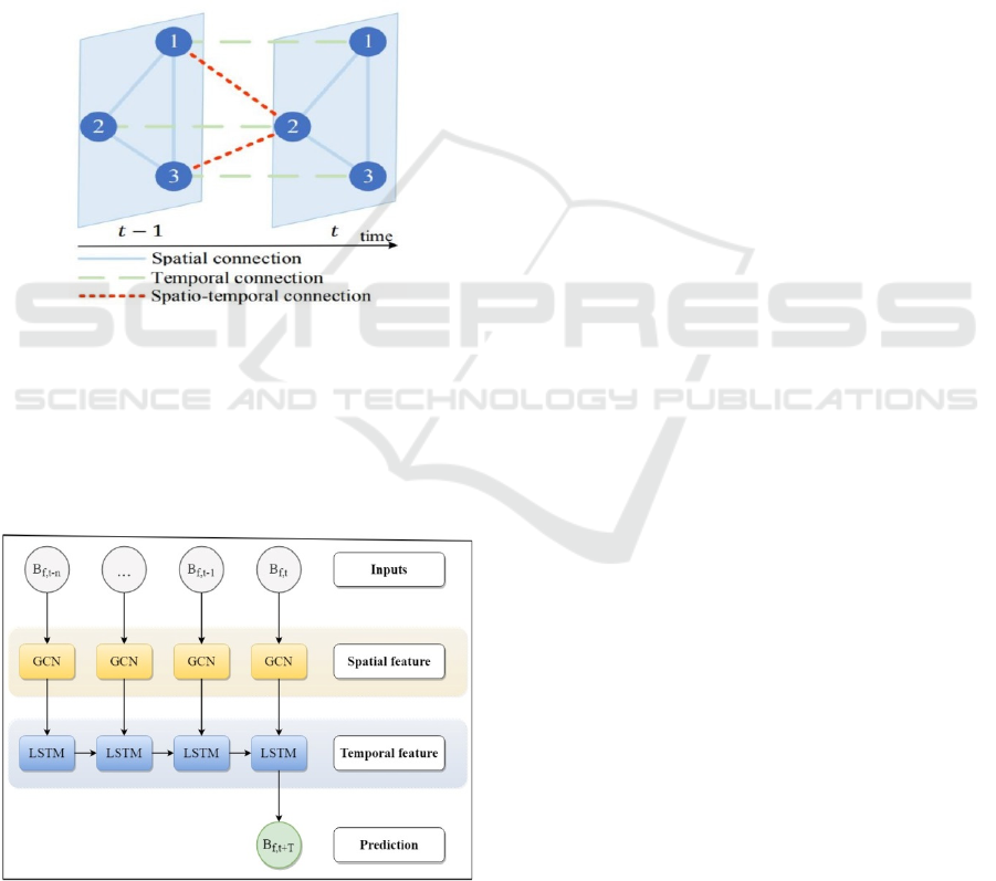
The key idea behind the construction of a spatio-

temporal neural network is illustrated in Figure 1.

Assume that the nodes 1,2,3 in the graph pictured

below represent three traffic sensors. A certain

traffic feature read by sensor 2 at timestamp 𝑡 may

explicitly be related (by spatial connections) to the

data read by sensors 1 and 3 at timestamp 𝑡, and to

the data read by sensor 2 at timestamp 𝑡1 (by the

temporal connection). Moreover, there exist implicit

spatio-temporal connections with the data read by

sensors 1 and 3 at timestamp 𝑡  1.

Figure 1: The spatial and temporal connections among

sensors arranged in a graph.

The architecture of the GCN-LSTM model

which is available as open source in the StellarGraph

library (CSIRO's Data61, 2018) was inspired by the

ideas proposed in (Zhao et al., 2020) and it is

illustrated in Figure 2.

Figure 2: The architecture of the GCN-LSTM model. For

each feature 𝑓 the 𝑆 time-series are used as input and the

final prediction is obtained by passing them through the

GCN and the LSTM layers.

According to (Zhao et al., 2020) and (CSIRO's

Data61, 2018) the GCN-LSTM model consists of

two distinct parts: the GCN layers and the LSTM

layers. The number and the size of GCN layers and

the LSTM layers, as well as the number of LSTM

cells are user defined. Remark that Gated Recurrent

Units (GRU) are used in (Zhao et al., 2020) instead

of LSTM, however in practice there are not any

significant differences between them and are equally

effective for various tasks. The basic operating

principles of both the GRU and LSTM are

approximately the same, according to (Chung et al.,

2020).

As can be seen in Figure 2, the GCN layers are

used first in order to capture the spatial relationships

between sensors. The information is added to the

(temporal) information contained by the inputted

time series. Remark that this part of the model can

be adapted for predicting the value of a certain

traffic feature on a future timestamp based only on

its current values across the sensors graph (at single

timestamp). However, the temporal information is

also very important for predictions, so for obtaining

the best results a subset of the time-series of values

of the traffic feature (as measured at several

previous timestamps across the sensors) should be

used in order to predict its value at a future

timestamp. For achieving this, in a second step the

time-series (now augmented with spatial features)

are inputted into the LSTM layers. (The number of

LSTM cells is given by the length of the subset of

the time-series used for training.) The final results

are obtained by passing through a dropout and a

dense layer. According to experimental results

(CSIRO's Data61, 2018), their usage leads to

improvement in performance and prevents over-

fitting.

In summary, the GCN-LSTM model may be

used for capturing both the spatial and the temporal

dynamics.

3.3 Dataset

For our experiments we have prepared a new dataset

using traffic data collected from various roads in the

State of California. The data is aggregated from

sensors positioned on the freeways of the state and it

is stored and publically available in the Caltrans

Performance Measurement System (PeMS, 2019), a

web platform where users can analyse and export

traffic information. The data was automatically

collected from the website using a Python script.

Since the PeMS data contains many sensors for

which the values of the corresponding features are

Predicting Multiple Trafﬁc Features using a Spatio-Temporal Neural Network Architecture

333

not measured, but instead are imputed by the system

or simply not available, one important step in

preparing the dataset was to choose several sensors

for which as many as possible real observed values

are available and which are also relatively close

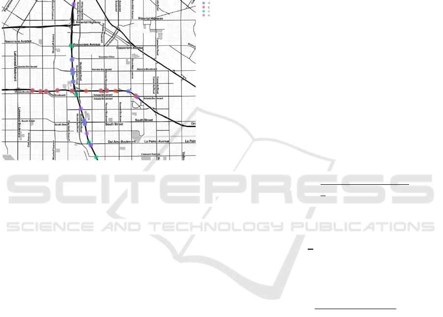
together. Using the plot on a map of the sensors and

their associated percentage of real observed values,

40 sensors found in all directions of a 4-way

interchange have been manually selected. They are

represented in Figure 1.

Figure 3: Map of the manually selected sensors. The

colours represent the corresponding traffic direction.

For the selected sensors, our dataset contains

time-series for all the traffic features studied in this

paper, i.e. flow, speed and occupancy. The time

period included in the dataset is from the 1

of April

to the 30

of April 2019. For each sensor

measurements are done every 5 minutes, so that a

full day of measurements contains 288 observations.

The system also offers a metadata file which

contains structured descriptions of each individual

sensor. From the data provided for each sensor the

following features are useful for computing spatial

information: freeway number, direction, latitude and

longitude.

3.4 Technical Implementation

For the implementation of the machine learning

models the Python libraries Tensorflow, Keras and

StellarGraph were used. Tensorflow (Google Brain,

2016) is a library developed by Google for

implementing machine learning applications. On top

of Tensorflow, another package has been built,

named Keras (Chollet, 2015). It contains

implementations of machine learning algorithms that

are very popular and may be used to define and train

models that combine them, as layers. StellarGraph

(CSIRO's Data61, 2018) is another library based on

TensorFlow that aims to help implementing graph

convolutional neural network architectures. The

open source implementation in StellarGraph of the

architecture proposed in (Zhao et al., 2020) was used

for the experiments presented in this paper.

4 EXPERIMENTS

4.1 Performance Metrics

For the purpose of measuring the performance of the

tested models, we have used in our experiments

three standard performance metrics that evaluate the

distance between the ground truth (i.e. the real, as

measured in traffic feature y

) and the computed

model prediction for the same feature. Assume that

the testing dataset contains 𝑁 samples (epochs) of

the form



𝑥



,𝑦





and 𝑚 is the model under

consideration. Denote by 𝑦



 the mean of 𝑦



.Then

the prediction of the model for 𝑦



is 𝑚



𝑥





and we

have:

 Root Mean Squared Error (RMSE):

𝑅𝑀𝑆𝐸



𝑚















𝑦



𝑚𝑥











;

 Mean Absolute Error (MAE):

𝑀𝐴𝐸



𝑚











𝑦



𝑚𝑥









;

 The Coefficient of Determination (R

𝑅





𝑚



1





𝑦



𝑚𝑥











∑

𝑦



𝑦













More precisely, the first two metrics are

measuring the model prediction error. They should

be interpreted as follows: the smaller is the number

computed, the better is the model. The capability of

the model to make good predictions is measured by

the coefficient of determination. Its interpretation is:

the closer to 1 is the number computed (by definition

it is always smaller than 1), the better is the model.

4.2 Tuning Model Parameters

For hyperparameters tuning a grid search is done in

order to find the best amount of hidden units on both

VEHITS 2022 - 8th International Conference on Vehicle Technology and Intelligent Transport Systems

334

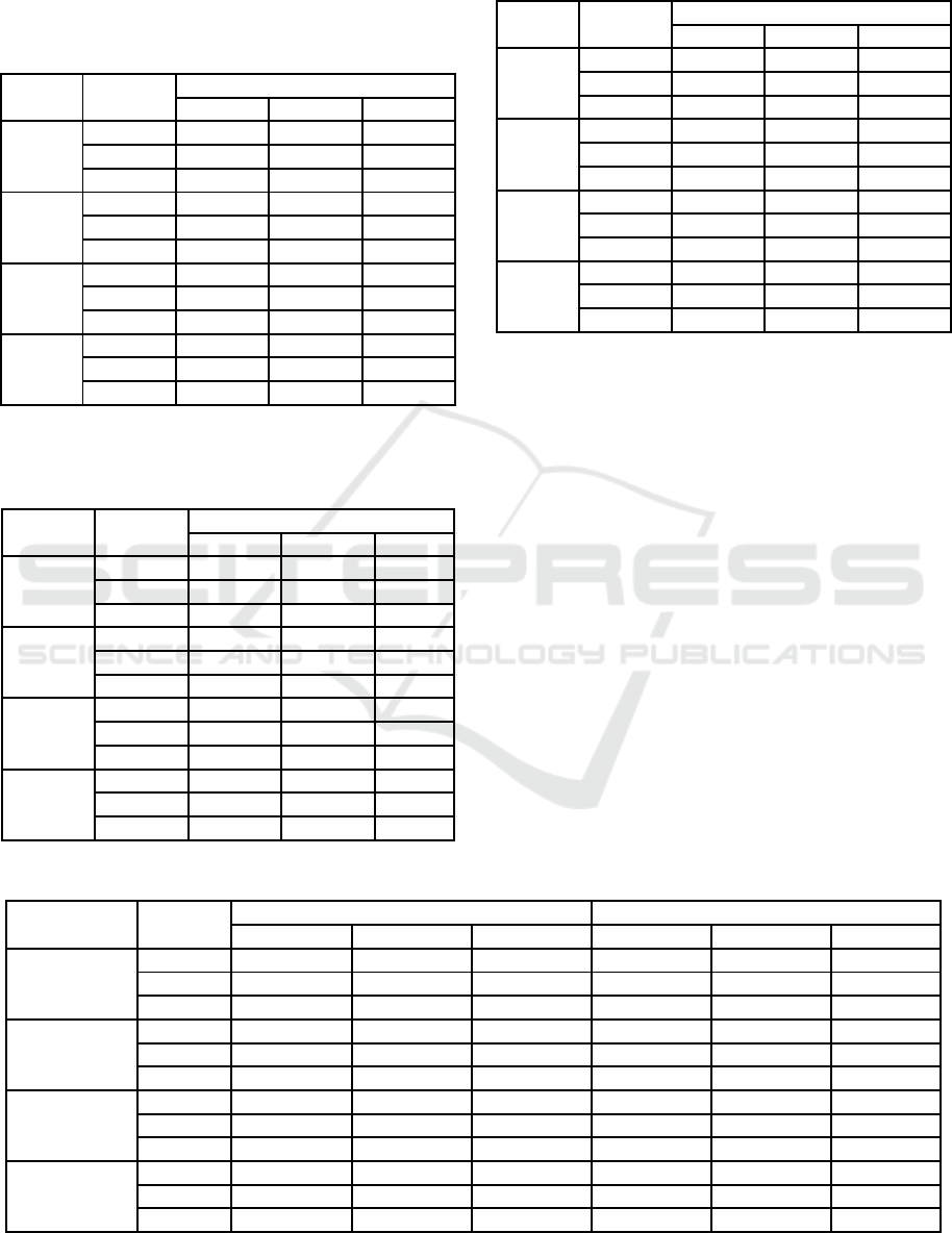
the GCN and the LSTM layers. The best settings are

automatically selected for making predictions.

Table 1: Measuring the GCN-LSTM performance for

predicting flow with variable amount of hidden units and

under different time horizons.

Time GCN

LSTM

64 128 256

15 min

16 25.55 21.69 22.88

32 23.97 23.38 21.18

64 24.45 22.57 21.51

30 min

16 28.29 26.80 27.22

32 31.55 27.85 26.24

64 26.66 25.74 24.86

45 min

16 30.99 27.56 28.49

32 29.41 28.50 28.27

64 29.39 30.06 29.02

60 min

16 33.55 34.70 32.50

32 32.78 33.71 30.36

64 33.36 29.87 30.33

Table 2: Measuring the GCN-LSTM performance for

predicting speed with variable amount of hidden units and

under different time horizons.

Time GCN

LSTM

64 128 256

15 min

16 51.90 51.77 48.74

32 50.00 49.10 46.48

64 48.95 49.76 43.60

30 min

16 80.46 74.87 77.11

32 82.95 78.08 72.43

64 79.29 77.48 75.94

45 min

16 95.26 94.33 97.12

32 95.75 93.23 93.94

64 96.05 94.80 90.07

60 min

16 111.20 106.79 123.63

32 110.45 107.35 111.23

64 117.64 106.60 114.93

Table 3: Measuring the GCN-LSTM performance for

predicting occupancy with variable amount of hidden units

and under different time horizons.

Time GCN

LSTM

64 128 256

15 min

16 27.91 24.51 25.28

32 27.37 24.46 24.58

64 26.53 24.86 22.64

30 min

16 31.42 30.81 30.26

32 31.80 30.04 30.37

64 31.70 30.75 30.45

45 min

16 34.97 34.08 34.10

32 34.23 34.65 34.46

64 34.66 33.50 35.28

60 min

16 38.43 37.98 38.95

32 37.35 37.43 37.34

64 38.25 36.74 36.07

The optimal number of hidden units found for

each feature and under each time horizon is marked

by bold numbers in the Tables 1, 2 and 3. Note that

the MSE numbers in these tables are scaled; smaller

numbers indicate better performance of the model.

4.3 Experimental Results

The performance of the GCN-LSTM model is

compared with the performance of a LSTM model

(Hochreiter et al., 1997), which is used as a baseline.

This allows us to see the combined spatio-temporal

prediction capability of the model.

The final results of our experiments are

contained in Table 4. We have compared the

predictions made by the two models for 4 times

horizons (15 min., 30 min., 45 min. and 60 min) and

for 3 different traffic features (flow, speed and

occupancy). From the total of 12 experiments made,

the GCN-LSTM model has provided better results

Table 4: Experimental Results.

Time Metric

LSTM GCN_LSTM

flow spee

occupanc

flow spee

occupanc

15 min

RMSE 48.7111 6.4772 0.0492 42.5435 7.117

0.0433

MAE 34.3575 3.5623 0.0273 30.5658 4.3369 0.0217

0.9396 0.8142 0.6452 0.9471 0.775

0.7253

30 min

RMSE 56.0602 9.5153 0.0549 46.9174 8.8095 0.0485

MAE 40.6417 5.4586 0.0329 34.1318 5.2449 0.0257

0.9077 0,5993 0.5568 0.9354 0.6566 0.6543

45 min

RMSE 62.9085 10.4843 0.0581 48.1666 8.9197 0.0499

MAE 47.1767 6.3406 0.0364 35.2929 5.5909 0.0278

0.8833 0.5139 0.5061 0.9319 0.6482 0.6342

60 min

RMSE 71.9628 11.5291 0.0609 51.2077 9.8415 0.0501

MAE 54.5468 7.6336 0.0394 37.9371 6.0044 0.0277

0.8466 0.4126 0.4548 0.9223 0.5720 0.6321

Predicting Multiple Trafﬁc Features using a Spatio-Temporal Neural Network Architecture

335

than the LSTM model in 11 experiments. There

exists 1 experiment (marked with italics in Table 4)

in which the results obtained with the LSTM model

were superior.

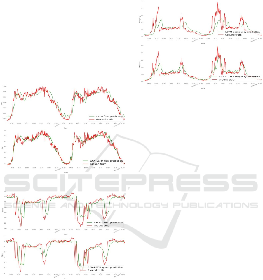
4.4 Visual Interpretation of the Results

For providing a better understanding of the results,

we have selected one particular sensor and the

predictions made by the two models for the 60

minutes time horizon on a 2-days subset of test set

are visualized in the Figures 2, 3 and 4.

Figure 4: LSTM and GCN-LSTM flow predictions.

Figure 5: LSTM and GCN-LSTM speed predictions.

Together with the numerical data for

performance in Table 4, these figures show:

 Especially over longer time horizons the more

complex spatio-temporal neural network

architecture has better prediction capability

than the simpler temporal neural network

architecture. In other words, adding the spatial

information to the model leads to a significant

improvement of its predictive power;

Figure 6: LSTM and GCN-LSTM occupancy predictions.

 The prediction performance depends on the

predicted traffic feature. As one can clearly

see by comparing Figures 2 and 3, as well as

from Table 4, there exist a difference in the

performance of both models for predicting

flow and speed. The flow predictions of both

models are significantly better than those for

speed.

5 CONCLUSIONS AND FUTURE

WORK

In this paper we present several experiments done

with a complex spatio-temporal neural network

architecture, which was initially proposed in (Zhao

et al., 2020), for 3 distinct traffic features and over 4

time horizons. First, we have found that, in almost

all cases, the predictive power of this new

architecture is superior to the one of a simpler

temporal model. We conclude that there exists

strong evidence that adding the spatial information is

very important. Second, unlike in the setup

considered in (Zhao et al., 2020) and also in other

related papers (where only one traffic feature is

investigated), we were interested to study the

performance of the architecture for various traffic

features, all of them being important for example

when building a modern traffic management system.

We have found that the architecture does not deliver

uniform performance across all traffic features, its

performance seem to depend heavily on the

particular feature used.

Our future work plan is to conduct more

experiments with several architectures proposed

very recently by various authors, as for example in

(Li et al., 2018), (Yu et al., 2018) and (Zhang et al.,

2020). We hope to find an architecture that does

VEHITS 2022 - 8th International Conference on Vehicle Technology and Intelligent Transport Systems

336

deliver uniform performance, independent on the

particular feature predicted. Since we have seen that

using spatial information in almost all studied cases

improves the overall performance of the model, we

also intend to experiment with new, better ways of

processing it.

ACKNOWLEDGEMENTS

This work was partially supported by a grant of the

Romanian Ministry of Education and Research,

CCCDI - UEFISCDI, project number PN-III-P2-2.1-

PTE-2019-0817, within PNCDI III.

REFERENCES

Atwood, J., Towsley, D. (2016). Diffusion-convolutional

neural networks. In NIPS'16, Proceedings of the 30th

International Conference on Neural Information

Processing Systems, 2001 – 2009.

Bruna, J., Zaremba, W., Szlam, A., LeCun, Y. (2014).

Spectral Networks and Locally Connected Networks

on Graphs. In ICLR 2014, Proceedings of the 2th

International Conference on Learning

Representations, pages 1 – 14.

Chollet, F., & others (2015). Keras. Available online at:

https://github.com/fchollet/keras.

Chung, J., Gulcehre, C., Cho, K., Bengio, Y. (2014).

Empirical Evaluation of Gated Recurrent Neural

Networks on Sequence Modeling. Presented in NIPS

2014, Deep Learning and Representation Learning

Workshop. Preprint arXiv: 1412.3555.

CSIRO's Data61 (2018). StellarGraph Machine Learning

Library. Online at https://stellargraph.readthedocs.io/.

Google Brain (2016). TensorFlow: A system for large-

scale machine learning. In OSDI'16, Proceedings of

the 12th USENIX conference on Operating Systems

Design and Implementation, pages 265 – 283.

Hechtlinger, Y., Chakravarti, P., Qin, J. (2017). A

generalization of convolutional neural networks to

graph-structured data. Preprint arXiv: 1704.08165.

Henaff, M., Bruna, J., LeCun, Y. (2015). Deep

convolutional networks on graph-structured data.

Preprint arXiv:1506.05163.

Hochreiter, S., Schmidhuber, J. (1997). Long short-term

memory. Neural Computation 9, pages 1735 – 1780.

Kipf, T., Welling, M. (2017). Semi-Supervised

Classification with Graph Convolutional Networks. In

ICLR 2017, Proceedings of the 6th International

Conference on Learning Representations, pages 1 –

14.

Li, Y., Yu, R., Shahabi, C., Liu, Y. (2018). Diffusion

Convolutional Recurrent Neural Network: Data-

Driven Traffic Forecasting. In ICLR 2018,

Proceedings of the 6th International Conference on

Learning Representations, pages 1 – 16.

Moravčík, M., Schmid, M., Burch, N., Lisý, V., Morrill,

D., Bard, N., Davis, T., Waugh, K., Johanson, M.,

Bowling, M. (2017). Deepstack: Expert-level artificial

intelligence in heads-up no-limit poker. Science 356,

pages 508 – 513.

Niepert, M., Ahmed, M., Kutzkov, K. (2016). Learning

convolutional neural networks for graphs. In ICML

2016, Proceedings of the 33rd International

Conference on Machine Learning, pages 2014 – 2023.

PeMS, Caltrans Performance Measurement System

(2019). Data avaible at https://pems.dot.ca.gov/.

Silver, D. et al. (2016). Mastering the game of go with

deep neural networks and tree search. Nature 529,

pages 484 – 489.

Silver, D. et al. (2017). Mastering the game of go without

human knowledge. Nature 550, pages 354 – 359.

Yu, B., Yin, H., Zhu, Z. (2018). Spatio-Temporal Graph

Convolutional Networks: A Deep Learning

Framework for Traffic Forecasting. In Proceedings of

the Twenty-Seventh International Joint Conference on

Artificial Intelligence, IJCAI-ECAI-2018, pages 3634

– 3640.

Zhang, Q., Chang, J., Meng, G., Xiang, S., Pan, C. (2020).

Spatio-Temporal Graph Structure Learning for Traffic

Forecasting. In Proceedings of the Thirty-Fourth AAAI

Conference on Artificial Intelligence, 1177 – 1185.

Zhao, L., Song, Y., Zhang, C., Liu, Y., Wang, P., Lin, T.,

Deng, M., Li H. (2020). T-GCN: A Temporal Graph

Convolutional Network for Traffic Prediction. IEEE

Transactions on Intelligent Transportation Systems

21, pages 3848 – 3858.

Predicting Multiple Trafﬁc Features using a Spatio-Temporal Neural Network Architecture

337