An Application of Scenario Exploration to Find New Scenarios for the

Development and Testing of Automated Driving Systems in Urban

Scenarios

Barbara Sch

utt

1 a

, Marc Heinrich

, Sonja Marahrens

, J. Marius Z

ollner

and Eric Sax

FZI Research Center for Information Technology, Karlsruhe, Germany

IPG Automotive GmbH, Karlsruhe, Germany

Keywords:

Advanced Driving Assistance Systems, Automated Driving, Scenario-based Testing, Scenario Exploration.

Abstract:

Veriﬁcation and validation are major challenges for developing automated driving systems. A concept that gets

more and more recognized for testing in automated driving is scenario-based testing. However, it introduces

the problem of what scenarios are relevant for testing and which are not. This work aims to ﬁnd relevant,

interesting, or critical parameter sets within logical scenarios by utilizing Bayes optimization and Gaussian

processes. The parameter optimization is done by comparing and evaluating six different metrics in two urban

intersection scenarios. Finally, a list of ideas this work leads to and should be investigated further is presented.

1 INTRODUCTION

The development of semi-automated, automated and

autonomous vehicles has played an important role in

the software and hardware departments of automotive

manufacturers during recent years. The consulting

company Gartner has already anticipated autonomous

things as a ”hot topic” several times in previous years

and is now going one step further. The current re-

port ”Top 10 Strategic Technology Trends for 2022”

predicts autonomic systems as a main area of inter-

est: systems that can not only make autonomous de-

cisions, but additionally are able to adapt and change

their behavior according to the environment (Gartner,

2021).

One type of autonomous or autonomic system are

automated vehicles. A major challenge besides their

development is to ensure that the system is sufﬁ-

ciently safe and can be approved and permitted on

public roads. A widely discussed testing approach

is scenario-based testing: According to (Otten et al.,

2018), one goal is to take realistic ﬁeld trial test drives

into simulation environments, where predeﬁned sce-

narios often serve as a basis for the derivation of rel-

evant test cases in automated assessment and, thus,

reducing the needed amount of real test drives. More-

over, the proper representation and usage of scenar-

ios during the development process support a seam-

https://orcid.org/0000-0001-8439-0322

less development and testing of automated driving

functions, as well as the speciﬁcation of requirements

and automated derivation of test cases (Bach et al.,

2016). However, the speciﬁcation of scenarios can in-

clude parameter ranges, where only a sub-set of these

ranges might bring insight into the performance of an

automated driving function or hold critical scenarios.

Additionally, introducing new parameters or parame-

ter ranges in a scenario increases the number of sce-

narios exponentially.

Novelty and Main Contribution to the

State of the Art

The novelty and main contribution of this paper is

a parameter evaluation for ﬁnding challenging and

critical scenario parameters in predeﬁned parameter

ranges. Thus, we

• optimize the parameters for different intersection

scenarios with different criticality metrics to ﬁnd

interesting scenarios and to save simulation time,

and

• use the information gained by the optimization

process to further assess these parameters and

their meaning for redeﬁning parameter ranges and

the evaluation and assessment of an automated

driving function.

338

Schütt, B., Heinrich, M., Marahrens, S., Zöllner, J. and Sax, E.

An Application of Scenario Exploration to Find New Scenarios for the Development and Testing of Automated Driving Systems in Urban Scenarios.

DOI: 10.5220/0011064600003191

In Proceedings of the 8th International Conference on Vehicle Technology and Intelligent Transport Systems (VEHITS 2022), pages 338-345

ISBN: 978-989-758-573-9; ISSN: 2184-495X

Structure

The paper is structured as follows: Section 2 brieﬂy

introduces topics related to this work, e.g., sce-

nario abstraction levels or Bayes optimization. Sec-

tion 3 explains the proposed exploration algorithm

and setup, including the simulation environment setup

and evaluation. In section 4, we conclude and give a

short overview of possible future work.

2 RELATED WORK

In the context of this work, the terms scenario and

scene are used as summarized by (Steimle et al.,

2021). A scene is a snapshots of a trafﬁc constella-

tion. A scenario is a sequence of scenes and describes

the temporal development of the behavior of different

actors within this sequence.

Finding new scenarios is a relevant step for deﬁn-

ing new test cases to assess an automated driving sys-

tem’s safety. (Bussler et al., 2020) use evolutionary

learning to ﬁnd relevant parameter sets within logical

scenarios and utilize Euclidean distance and time-to-

collision for their ﬁtness evaluation to ﬁnd more crit-

ical scenarios. Another approach proposed by (Bau-

mann et al., 2021) uses reinforcement learning com-

bined with the metrics headway and time-to-collision

to gain new test cases. Additionally, (Abeysirigoon-

awardena et al., 2019) use Bayes Optimization and

Euclidean distance to generate training scenarios for

a driving function to learn to avoid pedestrians by re-

inforcement learning. However, their work does not

produce a scenario set suitable for testing since their

approach always uses the current state of the driv-

ing function which changes over the course of the

experiments. Further, there are other approaches to

ﬁnd new scenarios, e.g., extracting scenarios from

recorded data sets as shown by (King et al., 2021)

and (Zofka et al., 2015) or by experts planning and

designing scenarios from scratch.

2.1 Scenario Abstraction Levels

(Menzel et al., 2018) suggest three abstraction levels

for scenario representation. The most abstract level

of scenario representation is called functional and de-

scribes a scenario via linguistic notation using natu-

ral, non-structured language terminology. The main

goal for this level is to create scenarios that are eas-

ily understandable and open for discussion between

experts. It describes the base road network and all

actors with their maneuvers, such as a right-turning

vehicle or road crossing cyclist. The next abstraction

level is the logical level and reﬁnes the representa-

tion of functional scenarios by a detailed represen-

tation with the help of state-space variables. These

variables or parameters can, for instance, be ranges

for road width, vehicle positions, and their speed, or

time and weather conditions. The most detailed level

is called concrete and describes operating scenarios

with concrete values for each parameter in the param-

eter space. Therefore, one logical scenario can yield

many concrete scenarios, depending on the number of

variables, size of parameter ranges, and step size for

these ranges.

2.2 Bayes Optimization and Gaussian

Process

Bayes optimization (BO) proceeds by maintaining a

global statistical model of a given objective func-

tion f (x) iteratively and consists of two main steps

(Greenhill et al., 2020): The ﬁrst step is the Gaus-

sian process, which is used to represent the predicted

mean µ

(x) and the uncertainty σ

(x) for each point

x of the input space, with the given set of observa-

tions D

1:t

= {(x

),(x

),...(x

)}, where x

the process input and y

the corresponding output at

time t. After that, an Acquisition function is used

to evaluate the beliefs about the objective function re-

garding the input space, based on the predicted mean

(x) and uncertainty and chooses the most promising

setting σ

(x).

2.3 Scenario Metrics

Scenario metrics are used to assess the quality of a

scenario regarding the aspect that needs to be eval-

uated. According to (Sch

utt et al., 2021), scenario

quality can be assessed at three different levels of res-

olution: nanoscopic (a scenario segment is evaluated,

e.g., a single time step), microscopic (a complete sce-

nario is evaluated, e.g., one concrete scenario), and

macroscopic (a set of scenarios is evaluated, e.g., a

logical scenario). Before a metric for the evaluation

process is chosen, the usage, goals, and purpose of

a scenario need to be clear, e.g., (Sch

onemann et al.,

2018) propose a hazard analysis and risk evaluation

to determine safety goals and show their approach on

the example of a valet parking system. The formu-

lated safety goals can be used in following steps to

choose the metrics for scenario evaluation or to deter-

mine the performance of an automated driving system

concerning its requirements.

An Application of Scenario Exploration to Find New Scenarios for the Development and Testing of Automated Driving Systems in Urban

Scenarios

339

2.4 Simulation Tools

Commercial tools for automotive simulation among

others are available from dSPACE (dSPACE, 2021),

and IPG (IPG Automotive GmbH, 2021). Both

simulation tools provide modules for map and sce-

nario creation, sensor models and dynamic models,

to name some examples. A further tool is Carla, an

open-source simulator with a growing community and

based on the game engine Unreal (Dosovitskiy et al.,

2017). It offers several additional modules, e.g., a sce-

nario tool which includes its own scenario format, a

graphical tool for creating scenarios, a ROS-bridge,

and SUMO support. SUMO is an open-source soft-

ware tool for modeling microscopic trafﬁc simulation

from DLR (Lopez et al., 2018). It specializes on big

scale of trafﬁc simulation and can be used for eval-

uating trafﬁc lights cycles, evaluation of emissions

(noise, pollutants), trafﬁc forecast, and many others.

3 DIRECTED SCENARIO

EXPLORATION

3.1 Optimization Setup

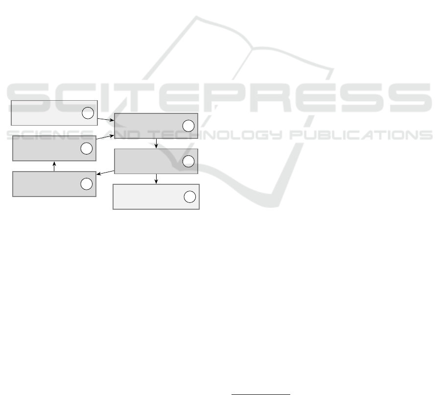
Start

parameter set

Simulation of

concrete scenario

Evaluation of

simulation results

Choose new

parameter set

Optimization

Termination

criterion met

Figure 1: Optimization workﬂow.

The optimization is an iterative process and is out-

lined in Fig. 1. First, a start parameter set is selected

(1), and simulated as summarized in step (2). The re-

sults are evaluated (3), a new parameter set is chosen

(5) by the optimization algorithm (4), and it is sim-

ulated again (2). This step is repeated until a termi-

nation criterion is met (6). The open-source project

common Bayesian optimization library (COMBO) is

employed in the experiments since it offers Bayesian

optimization that uses automatic hyperparameter tun-

ing, Thompson sampling as a method of picking the

next best candidate, and random feature maps for bet-

ter performance (Ueno et al., 2016). Throughout this

work, Bayesian optimization and Gaussian processes

were used. However, other optimization algorithms

might be used since the focus of this work does not

lie on the optimization itself.

3.2 Simulator Setup

The simulation tool CarMaker

serves as a basis for

the simulator setup (IPG Automotive GmbH, 2021).

As an open integration and test platform, CarMaker

provides a central control unit running the closed-

loop simulation. It includes all proprietary and exter-

nal models according to the given scenario and con-

straints. In this case, proprietary models of the com-

plete simulation environment comprise the road, en-

vironment and trafﬁc models. Six external models

were integrated as FMUs (Functional Mock-up Unit)

via an extended version of the Open Simulation Inter-

face (OSI) (ASAM OSI, 2021), realizing a setup with

three sensor models (camera, lidar (Linnhoff et al.,

2021), and radar), an autonomous driving function

(see section 3.3), a motion control model and a vehi-

cle dynamics model. This simulator setup is shown

in Fig 2. The output quantities of each simulation

are handed over to the optimization setup described in

section 3.1. The next scenario to be executed is then

chosen directly by the optimization setup via script

commands, leading to the optimization workﬂow pic-

tured in Fig 1.

3.3 Driving Function

To calculate the trajectory of the ego vehicle, a

lightweight and highly automated driving function

is used. The function is centered around a modi-

ﬁed, curvature-aware version of the Intelligent Driver

Model (IDM) as used in (Zofka et al., 2016), initially

introduced in (Treiber et al., 2000). To achieve a mod-

ular system, the function is implemented using the

Robot Operating System (ROS) framework (Quigley

et al., 2009). The system comprises six modules, as

shown in Fig. 3: a sensor fusion module to join the

information from the three sensors, a tracking algo-

rithm to keep track of occluded trafﬁc participants, a

ﬁlter module to extract the relevant objects, a routing

algorithm, a localization part to create an estimate of

the own global position using odometry information,

and ﬁnally, a trajectory module, planning a trajectory

with a velocity proﬁle.

The routing algorithm uses a high-deﬁnition map

to extract the road topology. The relevant objects

identiﬁed within the object ﬁlter are projected onto

the path of the ego vehicle. Thereby, a distance

and differential velocity can be calculated to be used

CarMaker from IPG Automotive in version 8.0.2

VEHITS 2022 - 8th International Conference on Vehicle Technology and Intelligent Transport Systems

340

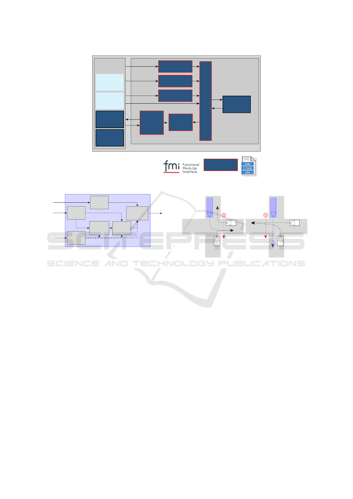
Simulation Setup

IPG

CarMaker

Simulation

Control

Logging

Engine

Trafﬁc

Models

Environment

Models

Camera Sensor

Lidar Sensor

Radar Sensor

HAD function proxy

Motion

Control

Vehicle

Dynamics

HAD

function

Simulation Models

TCP

Model FMU

Figure 2: Modular structure of the simulation environment.

Routing

Target

Position

Sensor

Fusion

Sensor

Information

Object

Tracking

Object

Filter

Trajectory

Planning

Trajectory

Local-

ization

Odometry

Figure 3: Modular structure of the driving function.

within the IDM. Filtering is done considering the type

of an object, as well as its position relative to the road

network and the ego vehicle. Moreover, the curvature

of the path is considered by converting it to a velocity

limit using maximum lateral acceleration. This veloc-

ity limit is treated as a separate object for the IDM to

achieve smooth cornering behavior.

A gateway architecture was used to comply with

the standardized FMI/OSI interface described in sec-

tion 3.2 while maintaining the platform’s indepen-

dence. Thereby, a TCP proxy was integrated into the

simulator as an FMU. The proxy forwards the mes-

sages via TCP to the communication layer of the driv-

ing function, where the messages are then converted

into equivalent ROS messages. With this, the driving

function can be run within a docker environment.

3.4 Logical Scenario

As shown in Fig. 4, two logical intersection scenarios

are used for the experiments. Each scenario consists

of an ego vehicle (E), a pedestrian (P), a second car

(C), and a truck (T). Both scenarios vary in the ac-

tors’ starting position and maneuvers. In scenario A,

Figure 4: Two experimental scenarios: a) ego turns right, b)

ego turns left. C: car, E: ego vehicle, P: pedestrian, T: truck.

the ego vehicle is turning right and, therefore, crosses

the trajectories of the pedestrian and the truck but not

the car’s trajectory, whereas, in scenario B, the ego ve-

hicle is turning left and crosses the trajectories of all

three adversary trafﬁc participants. The two scenarios

lead to different behaviors of the ego vehicle since it

reacts to other participants blocking its route. The fol-

lowing ranges were chosen as parameter ranges, for

which the optimal parameter sets have to be found

during the scenario exploration:

• Pedestrian Delay: The pedestrian waits for a

given time t

delay

in s before crossing the road,

where t

delay

∈ {0.0,...,7.0}. 50 samples with a

step size of 0.14s were taken.

• Ego Position: The ego vehicle starts at a given

s-coordinate s

start

in m along the road, where

start

∈ {27.99,...77.99}. 250 samples with a step

size of 0.2m were taken.

• Car Speed: The maximum speed v

max

that the

other car is allowed to achieve in m/s, where

max

∈ {12.5,...,30.0}. 50 samples with a step

An Application of Scenario Exploration to Find New Scenarios for the Development and Testing of Automated Driving Systems in Urban

Scenarios

341

size of 0.35m/s were taken.

This setup results in 625.000 scenarios. If each

scenario takes approximately 30 s for simulation ex-

ecution and calculation of criticality metrics, the ex-

ecution of all 625.000 scenarios takes more than 217

days of non-stop simulation on a single machine. Ad-

ditionally, the simulation time grows exponentially,

with scenarios getting more complex by additional

parameters and parameter ranges.

3.5 Optimization Problem

The goal of the scenario exploration is to ﬁnd all criti-

cal scenarios involving the ego vehicle and the pedes-

trian, the most vulnerable road user (VRU) in this sce-

nario. Therefore, the criticality between the ego vehi-

cle and the pedestrian is optimized. The criticality is

measured by criticality metrics, and the optimization

aims to ﬁnd scenarios evaluated to what degree they

contain a potentially critical situation. Five criticality

metrics were utilized as the objective function to be

optimized by the Bayesian optimization:

• Euclidean Distance: Direct distance between the

center of mass of two vehicles.

• Trajectory Distance: Distance between two traf-

ﬁc participants along their trajectories and road

network.

• Worst-time-to-collision (WTTC): Metricetric

based on time-to-collision (TTC) (Hayward,

1972), but without the TTC’s limitation to car fol-

lowing scenarios (Wachenfeld et al., 2016).

• Gap Time (GT): The predicted distance in time

between the two trafﬁc participants crossing an in-

tersection (Allen et al., 1978).

• Post-encroachment-time (PET): The actual dis-

tance in time between the two trafﬁc participants

crossing an intersection (Allen et al., 1978).

All metrics above require to minimize their out-

put value to optimize the criticality within the logical

scenario.

3.6 Experiments and Results

All experiments evaluate the criticality of the scenario

regarding the ego vehicle and the pedestrian as the

most VRU in this scenario. Some scenarios might

lead to critical situations between the ego vehicle and

other trafﬁc participants. However, these scenarios

are neglected. In general, different metrics cannot be

compared directly, e.g., a critical scenario in Fig 6 b)

which is indicated by a red dot is not equally critical

to a red colored scenario in Fig 6 c).

distance in m

pedestrian delay in s

Scenario A

Scenario B

time in s

Euclid. Distance [m]

Trajectory Distance [m]

Gap Time [s]

PET [s]

WTTC [s]

0.0

0 1 2

4 5 6 7

0 1 2 3

5 6 7

2.5

5.0

7.5

10.0

Figure 5: Bayes optimization results of both scenarios on a

one-dimensional parameter space. The metrics used for op-

timization are Euclidean and trajectory distance, gap time,

post-encroachment-time, and worst-time-to-collision.

3.6.1 Experiment 1

In the ﬁrst set of experiments, only the pedestrian

delay is varied and optimized throughout all simula-

tions, with a set value of s

start

= 60.0 m in scenario

A, s

start

= 67.0 m in scenario B, and v

max

= 15.0 m/s

in both scenarios. The results are shown in Fig. 5 a)

for scenario A and in b) for scenario B. In scenario

A, critical scenarios are found for a delay near 0.0 s,

and for all metrics except PET, there are no changes

in criticality for a delay over approximately 1.5s. Al-

though PET values change after that, scenarios are not

critical since the result is growing. Further, (Allen

et al., 1978) set the threshold for critical scenarios to

PET < 1.5 s. The used criticality metrics in scenario

B indicate no change in criticality for a varying pedes-

trian delay, and therefore, the pedestrian delay has no

inﬂuence on the outcome of scenario B for the chosen

values of the other two parameters.

3.6.2 Experiment 2

In the second setup, all three parameters are varied

and optimized as described in section 3.1 and 3.4.

The results for these experiments are shown in Fig. 6,

where a) shows results for the Euclidean distance,

b) trajectory distance, c) post-encroachment-time, d)

worst-time-to-collision, and e) gap time. In both sce-

narios, the car speed seems to have no or almost no

visible inﬂuence on simulation results regarding the

criticality of the pedestrian’s situation. Therefore, a

three-dimensional plot can be reduced to the two di-

mensions of pedestrian delay and ego s-coordinate.

However, this does not mean that there is no inﬂuence

at all, and outliers or deviations in the plot that are not

congruent with other values around them might be in-

ﬂuenced by the car’s speed. An explanation for the

VEHITS 2022 - 8th International Conference on Vehicle Technology and Intelligent Transport Systems

342

Scenario A

Scenario A Scenario A Scenario A

Scenario B Scenario B Scenario B Scenario B Scenario B

ego s-coordinate in m ego s-coordinate in m

ego s-coordinate in m ego s-coordinate in m ego s-coordinate in m

ego s-coordinate in m ego s-coordinate in m ego s-coordinate in mego s-coordinate in m

ego s-coordinate in m

pedestrian delay in s

40 60 80

2.5

2.0

4.0

3.0

3.5

0.4

0.2

1.0

0.6

0.8

0.2

0.1

0.6

0.5

0.3

0.4

pedestrian delay in s

pedestrian delay in s pedestrian delay in s

pedestrian delay in spedestrian delay in s

40 60 80 40 60 80 40 60 80 40 60 80

40 60 80 40 60 80 40 60 80

40 60 80

Euclidean Distance in m

Trajectory Distance in m

Post-Encroachment-Time in s Post-Encroachment-Time in s

Worst-Time-To-Collision in s Worst-Time-To-Collision in s

Gap Time in s

e)d)

Figure 6: Bayes optimization results of both scenarios on a three-dimensional parameter space. The metrics used for opti-

mization are Euclidean (a) and trajectory (b) distance, post-encroachment-time (c), worst-time-to-collision (d), and gap time

(e) and are shown in a two-dimensional space since the variable car speed has almost no inﬂuence on the scenario outcome.

Figure 7: Screenshot from a less critical scenario (left)

and critical scenario where the ego vehicle almost hits the

pedestrian (right).

lack of inﬂuence could be, that in scenario A, the ego

vehicle’s trajectory and the car’s trajectory are not in-

tersecting, and the ego has no need to react to the car.

Also, the other car is starting close to the intersec-

tion in both scenarios, it might simply not have had

enough time to accelerate until it reaches the inter-

section and always pass the ego vehicle at the same

speed.

In general, scenario A has three different out-

comes regarding the criticality of the pedestrian’s sit-

uation: the ego vehicle reaches the intersection and

stops for the pedestrian who is crossing the street.

This result can be observed in scenarios at the bot-

tom left corner in Fig. 6 a)-e) where the criticality de-

creases for most metrics. The second result consists

of the ego vehicle passing the intersection before the

pedestrian or the truck, which are mostly scenarios at

the top half and right half in Fig 6 a)-e). The last vari-

ant are scenarios where the ego vehicle reaches the

intersection right after the truck and, therefore, can-

not see the pedestrian. These scenarios are the criti-

cal scenarios around the diagonal near the bottom left

corner in Fig. 6 a)-e).

In scenario B, the ego vehicle not only reacts to

the pedestrian and the truck but also the other car. The

outcomes of scenario B are the same as in scenario A.

However, they are distributed differently over the pa-

rameter space: the less critical area in the bottom left

corner, which can be clearly observed in Fig. 6 b) and

d) results from a parameter set, where the ego vehicle

intersects the pedestrian’s path after they crossed the

road. The left part of Fig. 7 shows a screenshot of this

situation taken during the simulation. On the right

side, where the s-coordinate has its highest value, the

ego vehicle passes the intersection before the pedes-

trian, followed by a critical line around 70 m with

near-collisions. In the middle and left part of the s-

coordinate, the ego vehicle waits for the pedestrian to

pass, and the critical cluster at delay 2 s results from

interference with the truck.

The comparison of the results of both scenarios

leads to the following conclusions:

• Scenario A has a higher variance in criticality than

scenario B,

• car speed has no recognizable inﬂuence in sce-

nario A and almost no inﬂuence in B,

• some metrics are more sensitive, e.g., trajectory

distance and gap time, and

• some metrics lead to similar patterns in criticality,

e.g., bottom left corner in scenario A or scenar-

ios with a small ego vehicle s-coordinate in sce-

nario B.

3.6.3 Experiment 3

In the third setup, the pedestrian delay t

delay

is re-

placed by a new variable y

start

to see if the car speed

has more inﬂuence on the scenario outcome:

• Car Position: The y-coordinate y

start

in m fulﬁls

An Application of Scenario Exploration to Find New Scenarios for the Development and Testing of Automated Driving Systems in Urban

Scenarios

343

Scenario B

car speed in m/s

ego s-coordinate

in m

car y-coordinate in m

Post-Encroachment-Time in s

Figure 8: Exemplary Bayes optimization results of scenario

B on a three-dimensional parameter space for the metric

post-encroachment-time.

start

∈ {15.0, ..., 50.0}. 50 samples with a step

size of 0.7m were taken.

All three variables are varied and optimized, and the

ﬁve previously mentioned metrics are used. The re-

sults for scenario A do not show any inﬂuence of the

car’s speed or y position on the outcome. This is not

surprising since there is no trajectory intersection be-

tween the ego vehicle and the car. The results show,

the outcome only depends on the s-coordinate. As

Fig. 8 shows, in scenario B the ego s-coordinate still

has the most inﬂuence on the outcome. However, in

some areas in the parameter space car speed and y-

coordinate also affect the scenario criticality.

3.7 Results

In our experiments, we could show that even though

different metrics were used, they led to similar crit-

ical scenario clusters although, these metrics are not

comparable in the severity of the measured criticality

and their sensitivity. Moreover, our approach led to a

reduction of the amount of necessary simulation: in-

stead of executing more than half a million scenarios,

only about 430 were executed in experiments 2 and

3, respectively. Additionally, we were able to show

that the variable car speed has no inﬂuence in sce-

nario A and can be neglected to reduce the number of

scenarios or replaced by another variable with more

inﬂuence.

4 CONCLUSION AND FUTURE

WORK

In this work, we used an optimization algorithm to

ﬁnd critical scenarios for the develoing and testing

of automated and highly automated driving systems.

Bayes optimization with Gaussian process was uti-

lized in combination with ﬁve criticality metrics from

the automotive domain to calculate the process out-

put. This approach was used in two different experi-

ments and evaluated accordingly.

Derived from the evaluation of the experiments

and the results of this work, additional questions arise.

Results of the same scenario, models, criticality met-

rics, and the same driving function could be used

by different simulation tools and compared regard-

ing their deviation. Furthermore, it is harder to mea-

sure criticality for other scenarios, i.e., scenarios with

more trafﬁc participants. Our experiments only fo-

cused on criticality metrics between the ego vehicle

and the most VRU, the pedestrian. However, such a

choice might not always be obvious or changing dur-

ing one scenario, e.g., in urban rush hour trafﬁc with a

high density of trafﬁc participants. Metrics to evaluate

the relation between the ego and more than one adver-

sary trafﬁc participant or the whole scenario situation

are needed to make more objective conclusions. In

future work, the problem of ﬁnding more objective

metrics for scenarios will be approached to be able to

ﬁnd critical situations between the ego vehicle and the

sum of all other trafﬁc participants.

ACKNOWLEDGEMENTS

This research is funded by the “Simulations-

basiertes Entwickeln und Testen von automatisiertem

Fahren (SET Level)-Simulation-Based Development

and Testing of Automated Driving,” a succes-

sor project to the project “Projekt zur Etablierung

von generell akzeptierten G

utekriterien, Werkzeu-

gen und Methoden sowie Szenarien und Situatio-

nen zur Freigabe hochautomatisierter Fahrfunktionen

(PEGASUS)” and a Project in the PEGASUS Family,

promoted by the German Federal Ministry for Eco-

nomic Affairs and Energy (BMWi) under the grant

number 19 A 19004.

REFERENCES

Abeysirigoonawardena, Y., Shkurti, F., and Dudek, G.

(2019). Generating adversarial driving scenarios in

VEHITS 2022 - 8th International Conference on Vehicle Technology and Intelligent Transport Systems

344

high-ﬁdelity simulators. In 2019 International Con-

ference on Robotics and Automation (ICRA), pages

8271–8277. IEEE.

Allen, B. L., Shin, B. T., and Cooper, P. J. (1978). Analysis

of trafﬁc conﬂicts and collisions. Technical report.

ASAM OSI (2021). ASAM OSI

 (Open Simulation Inter-

face). Accessed: Dec. 15, 2021.

Bach, J., Otten, S., and Sax, E. (2016). Model based sce-

nario speciﬁcation for development and test of auto-

mated driving functions. In 2016 IEEE Intelligent Ve-

hicles Symposium (IV), pages 1149–1155. IEEE.

Baumann, D., Pfeffer, R., and Sax, E. (2021). Auto-

matic generation of critical test cases for the devel-

opment of highly automated driving functions. In

2021 IEEE 93rd Vehicular Technology Conference

(VTC2021-Spring), pages 1–5. IEEE.

Bussler, A., Hartjen, L., Philipp, R., and Schuldt, F. (2020).

Application of evolutionary algorithms and critical-

ity metrics for the veriﬁcation and validation of auto-

mated driving systems at urban intersections. In 2020

IEEE Intelligent Vehicles Symposium (IV), pages 128–

135. IEEE.

Dosovitskiy, A., Ros, G., Codevilla, F., Lopez, A., and

Koltun, V. (2017). CARLA: An open urban driving

simulator. In Proceedings of the 1st Annual Confer-

ence on Robot Learning, pages 1–16.

dSPACE (2021). SIMPHERA - Web-based solution for

simulation and validation in autonomous driving de-

velopment. Accessed: Jan. 19, 2022.

Gartner (2021). Top strategic technology trends

for 2022. https://www.gartner.com/en/information-

technology/insights/top-technology-trends. Accessed:

2021-10-25.

Greenhill, S., Rana, S., Gupta, S., Vellanki, P., and

Venkatesh, S. (2020). Bayesian optimization for adap-

tive experimental design: A review. IEEE Access,

8:13937–13948.

Hayward, J. C. (1972). Near miss determination through

use of a scale of danger. In Unknown. Publisher:

Pennsylvania State University University Park.

IPG Automotive GmbH (2021). CarMaker. Accessed: Dec.

20, 2021.

King, C., Braun, T., Braess, C., Langner, J., and Sax, E.

(2021). Capturing the variety of urban logical sce-

narios from bird-view trajectories. In VEHITS, pages

471–480.

Linnhoff, C., Rosenberger, P., and Winner, H. (2021). Re-

ﬁning object-based lidar sensor modeling — challeng-

ing ray tracing as the magic bullet. IEEE Sensors Jour-

nal, 21(21):24238–24245.

Lopez, P. A., Behrisch, M., Bieker-Walz, L., Erdmann, J.,

otter

od, Y.-P., Hilbrich, R., L

ucken, L., Rummel, J.,

Wagner, P., and Wießner, E. (2018). Microscopic traf-

ﬁc simulation using sumo. In The 21st IEEE Interna-

tional Conference on Intelligent Transportation Sys-

tems. IEEE.

Menzel, T., Bagschik, G., and Maurer, M. (2018). Scenarios

for development, test and validation of automated ve-

hicles. In 2018 IEEE Intelligent Vehicles Symp. (IV),

pages 1821–1827. IEEE.

Otten, S., Bach, J., Wohlfahrt, C., King, C., Lier, J., Schmid,

H., Schmerler, S., and Sax, E. (2018). Automated

assessment and evaluation of digital test drives. In

Advanced Microsystems for Automotive Applications

2017, pages 189–199. Springer.

Quigley, M., Conley, K., Gerkey, B., Faust, J., Foote, T.,

Leibs, J., Wheeler, R., Ng, A. Y., et al. (2009). Ros: an

open-source robot operating system. In ICRA work-

shop on open source software, volume 3, page 5.

Kobe, Japan.

Sch

onemann, V., Winner, H., Glock, T., Otten, S., Sax, E.,

Boeddeker, B., Verhaeg, G., Tronci, F., and Padilla,

G. G. (2018). Scenario-based functional safety for

automated driving on the example of valet parking.

In Future of Information and Communication Confer-

ence, pages 53–64. Springer.

Sch

utt, B., Steimle, M., Kramer, B., Behnecke, D., and

Sax, E. (2021). A taxonomy for quality in simulation-

based development and testing of automated driving

systems. arXiv preprint arXiv:2102.06588.

Steimle, M., Menzel, T., and Maurer, M. (2021). To-

wards a consistent terminology for scenario-based de-

velopment and test approaches for automated vehi-

cles: A proposal for a structuring framework, a ba-

sic vocabulary, and its application. arXiv preprint

arXiv:2104.09097.

Treiber, M., Hennecke, A., and Helbing, D. (2000). Con-

gested trafﬁc states in empirical observations and mi-

croscopic simulations. Phys. Rev. E, 62:1805–1824.

Ueno, T., Rhone, T. D., Hou, Z., Mizoguchi, T., and Tsuda,

K. (2016). Combo: an efﬁcient bayesian optimiza-

tion library for materials science. Materials discovery,

4:18–21.

Wachenfeld, W., Junietz, P., Wenzel, R., and Winner, H.

(2016). The worst-time-to-collision metric for situa-

tion identiﬁcation. In 2016 IEEE Intelligent Vehicles

Symposium (IV), pages 729–734. IEEE.

Zofka, M. R., Kuhnt, F., Kohlhaas, R., Rist, C., Schamm, T.,

and Z

ollner, J. M. (2015). Data-driven simulation and

parametrization of trafﬁc scenarios for the develop-

ment of advanced driver assistance systems. In 2015

18th International Conference on Information Fusion

(Fusion), pages 1422–1428. IEEE.

Zofka, M. R., Kuhnt, F., Kohlhaas, R., and Z

ollner, J. M.

(2016). Simulation framework for the development of

autonomous small scale vehicles. In 2016 IEEE In-

ternational Conference on Simulation, Modeling, and

Programming for Autonomous Robots, SIMPAR 2016,

San Francisco, CA, USA, December 13-16, 2016,

pages 318–324.

An Application of Scenario Exploration to Find New Scenarios for the Development and Testing of Automated Driving Systems in Urban

Scenarios

345