
Global Spare Parts Exploitation Costs Optymization and Its Reduction
to Rectangular Knapsack Problem
Andrzej Chmielowiec
1 a
, Leszek Klich
1 b
, Weronika Wo
´
s
1 c
and Adam Błachowicz
2 d
1
Faculty of Mechanics and Technology, Rzeszow University of Technology, Kwiatkowskiego 4, Stalowa Wola, Poland
2
Pilkington Automotive Poland, Strefowa 17, Chmiel
´
ow, Poland
Keywords:
Maintenance, Cost Optimization, Weibull Distribution, Exploitation Costs, Manufacturing Execution System,
Knapsack Problem.
Abstract:
Maintenance costs represent a significant portion of the budget in large enterprises. Unplanned downtime and
breakdowns have a very negative impact on the financial result. Minimizing their number is today a huge chal-
lenge for systems supporting production management and maintenance processes. Due to intensive research
in the field of reliability today, we know a lot about the optimal use of a single spare part. Unfortunately, the
analytical methods used for this purpose do not work well in the case of simultaneous analysis of the entire
production line. The article proposes a combination of analytical methods and discrete optimization methods
for global management of spare parts operating costs. The purpose of the presented algorithm is to support
decision-making that minimize the global cost of maintaining reliability in the entire production company.
1 INTRODUCTION
Despite the installation of an increasing number of
sensors and monitoring the degree of wear of many
systems and their subassemblies, there is still a large
number of elements which usability status is de-
termined in a binary manner: functional / non-
functional. An example is an oil hose for which the
performance level on the fly cannot be determined.
Perhaps in the future, advanced vision systems will be
able to automatically detect microcracks on its surface
and track wear levels. At present, however, the opera-
tion of such cases is purely reactive. The exchange
is made at a strictly defined moment or the failure
is removed when it occurs. From the point of view
of maintenance people, this is a rather uncomfortable
situation. However, for each such element on the pro-
duction line, we can determine the optimum working
time. Optimum time is understood here as the time
that minimizes the costs of servicing. Intuition sug-
gests that if the removal of a failure is much more
expensive than a scheduled replacement, the standard
working time of such an element should be shorter
a
https://orcid.org/0000-0001-6629-0029
b
https://orcid.org/0000-0001-6099-2417
c
https://orcid.org/0000-0003-4709-4369
d
https://orcid.org/0000-0003-4465-2652
than in a situation where the costs of removing a fail-
ure and scheduled replacement are similar. However,
the question is: when should the replacement be made
so that the long-term costs are as low as possible?
This problem will be discussed in this article. In the
following parts, it will be shown how modern IT tools
combined with the classical theory of reliability can
support the decision-making process in a manufactur-
ing company.
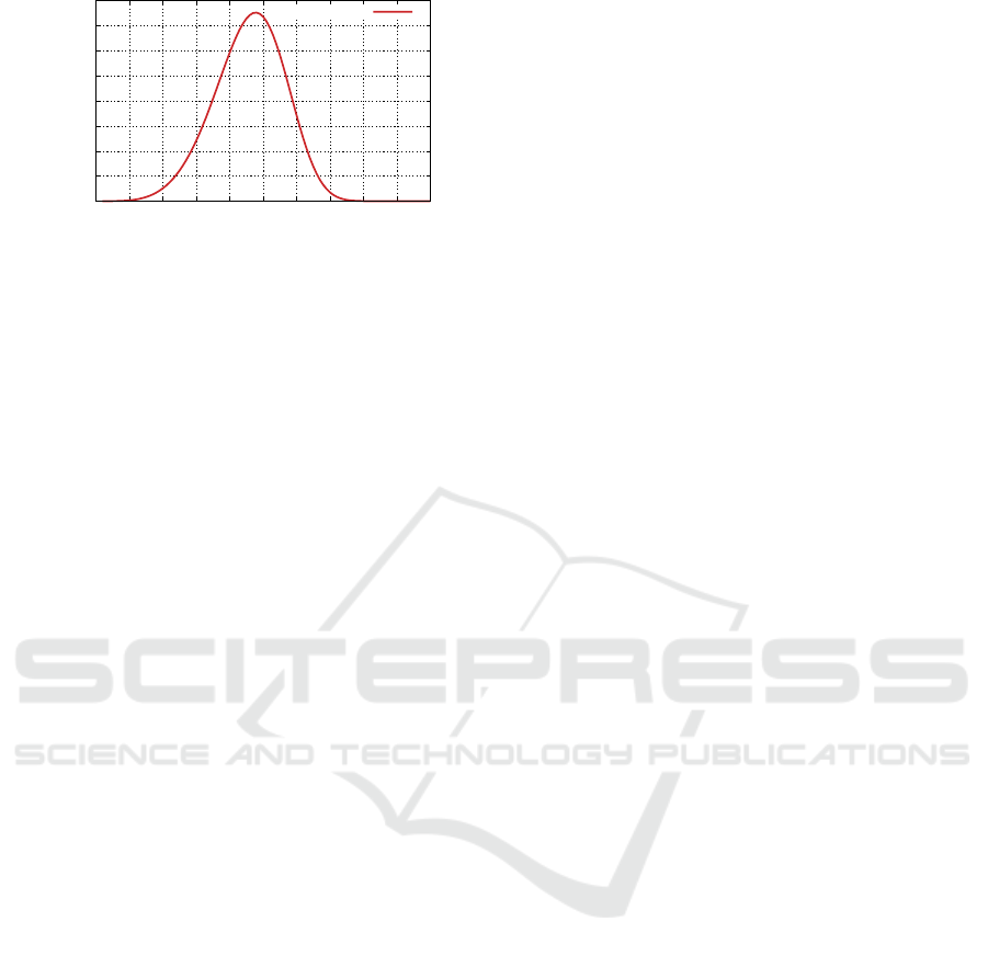
The Figure 1 shows the Weibull distribution with
parameters of α = β = 5, respectively. This distri-
bution was chosen as an example to illustrate the re-
liability of aging components. In practice, for each
element, the α and β parameters should be estimated
based on historical data (which will be presented in
the following sections) or information from the man-
ufacturer. It can be calculated that the average prod-
uct lifetime for a distribution with these parameters is
about 4.6 time units (e.g. months).
The Figure 1 shows that the systematic replace-
ment of such an element every one time unit prac-
tically eliminates the problem of failure. Therefore,
the manufacturer may recommend that users regularly
replace them at a specific time period. However, is
this approach economically justified? Unfortunately,
there is no clear answer to this problem. The solu-
tion depends on the cost of replacing this element dur-
ing standard service activities, and the cost of replace-
364
Chmielowiec, A., Klich, L., Wo
´
s, W. and Błachowicz, A.
Global Spare Parts Exploitation Costs Optymization and Its Reduction to Rectangular Knapsack Problem.
DOI: 10.5220/0011067400003179
In Proceedings of the 24th International Conference on Enterprise Information Systems (ICEIS 2022) - Volume 1, pages 364-373
ISBN: 978-989-758-569-2; ISSN: 2184-4992
Copyright
c
2022 by SCITEPRESS – Science and Technology Publications, Lda. All rights reserved
0
0.05
0.1
0.15
0.2
0.25
0.3
0.35
0.4
0 1 2 3 4 5 6 7 8 9 10
Failure PDF
Time
α=5, β=5
Figure 1: Probability density for the Weibull distribution
with α = 5 and β = 5.
ment in the event of a failure. It should be emphasized
that the costs related to downtime should be added to
the cost of the service replacement as well as to the
cost of the replacement during a failure. This is a very
important cost component that can cause the same el-
ement used at different points in the production line
to be treated differently. In fact, any finite resource at
the company’s disposal that has any value can be con-
sidered as a cost. This can be time, money, energy,
etc. In principle, cost should be understood to mean
all the necessary resources that are consumed during
replacement (both service replacement and failure re-
placement).
The problem of age replacement policy is the sub-
ject of many authors’ publications. First (Barlow and
Proschan, 1965) and (Barlow and Proschan, 1975)
have analyzed the optimization of the expected op-
erating costs and the impact of the replacement pol-
icy on these costs. Moreover, for several common
failure distributions methods have been developed by
(Glasser, 1967). On the other hand, (Fox, 1966) and
(Ran and Rosenlund, 1976) consider the optimal re-
placement time, taking into account discounting - this
issue is especially important in the case of rapidly
changing prices. The publications (Scmeaffer, 1971),
(Cl
´
eroux and Hanscom, 1974), (Cl
´
eroux et al., 1979)
and (Subramanian and Wolff, 1976) present a gener-
alized approach to the optimization of operating costs
and preventive replacement. The confidence intervals
with unknown failure distributions for the problem of
minimizing the expected replacement costs were also
quite intensively investigated, which can be found in
the articles (Ingram and Scheaffer, 1976), (Frees and
Ruppert, 1985), (L
´
eger and Cl
´
eroux, 1992). Next,
(Berg and Epstein, 1978) compares an age-related ex-
change policy with exchange policy at strictly defined
periods. The articles (Christer, 1978) and (Ansell
et al., 1984) analyze the asymptotic operating costs
assuming the replacement policy according to the age
of the element. A very extensive bibliography on the
problem of optimization of maintenance costs was
presented by (Nakagawa, 2003). In the review arti-
cle (Zhao et al., 2017) an up-to-date summary of the
state of knowledge in this field and perspectives for
further research directions can be found. It should
be emphasized that the problem of the replacement
policy as a result of aging is also valid today, as evi-
denced by publications from recent years (Knopik and
Migawa, 2017), (Fu et al., 2018), (Finkelstein et al.,
2020), (Wang et al., 2021a), (Zhao et al., 2021). One
problem in the practical use of the methods devel-
oped so far is focusing attention on a single element
or spare part. In this article, a global approach will
be proposed, the aim of which will be to optimize the
expected operating costs of the entire production line.
For this reason, under certain assumptions, analyti-
cal methods will be combined with discrete optimiza-
tion methods reducing the problem to a two- or one-
dimensional knapsack problem.
2 MINIMAL OPERATING COST
FOR SINGLE ELEMENT
The problem of optimal selection of the replacement
time will be presented in a more formal way. Let C
F
be the cost of removing the failure of a given element,
and C
M
the cost of the scheduled service replacement.
Moreover, let a = C
F
/C
M
. In addition, it is assumed
that C
F
= C
M
+ τ C
D
, where C
D
is the downtime cost
per unit of time and τ is the downtime required dur-
ing a failure. It follows from the assumptions that the
coefficient a > 1. It is then assumed that there will
be regular maintenance replacements for this item at
exactly T units of time since the previous replace-
ment. If F(t) is the failure probability at time t, and
G(t) = 1−F(t) is the reliability at time t, then the ex-
pected cost of service activities for the given replace-
ment time T is estimated as
C
T
= C
F
F(T ) +C
M
G(T ). (1)
In the formula above, the cost C
T
is simply the
weighted average cost of failure C
F
that occurs with
probability F(T ) and service cost C
M
that occurs with
probability G(T ) = 1 − F(T ). If we consider that
C
F
= a ·C
M
, we get the following equality
C
T
= C
M
1 + (a − 1)F(T )
. (2)
The calculated cost C
T
is not enough. It does not
yet take into account the frequency with which such
changes will be made. There may be a situation in
which the average cost of C
T
is small, but the fre-
quency with which it will be borne is so high that it
is not an optimal solution. So let µ
T
denote the mean
time between replacements of a given element, both
Global Spare Parts Exploitation Costs Optymization and Its Reduction to Rectangular Knapsack Problem
365
due to the failure and the planned service replace-
ment. Then the value µ
−1
T
determines the frequency
of replacement of the element and allows to define
the ε
T
function which expresses the relative cost of
maintaining the efficiency of the element per unit of
time
ε
T
=
C
T
C
M
· µ
−1
T
. (3)
Minimizing the ε
T
function is our main task. Before
we get down to that, it is necessary to define the for-
mula for the expected replacement time µ
T
. It is given
by the following formula (Nakagawa, 2006)
µ
T
=
T
Z
0
t dF(t) + T G(T ) =
T
Z
0
G(t) dt. (4)
Thus, the ε
T
function defining the relative cost of
maintaining efficiency per unit of time is expressed
as follows
ε
T
=
1 + (a − 1)F(T )
T
R
0
G(t) dt
. (5)
Nakagawa (Nakagawa, 2003) showed that T minimiz-
ing the value of ε
T
meets one of the following condi-
tions:
1. is finite and is given uniquely,
2. is infinite.
0
1
2
3
4
5
6
7
0 1 2 3 4 5 6 7 8 9 10
Relative cost of maintaining efficiency
per unit of time ε
T
Time
a=2
a=4
a=8
a=16
a=32
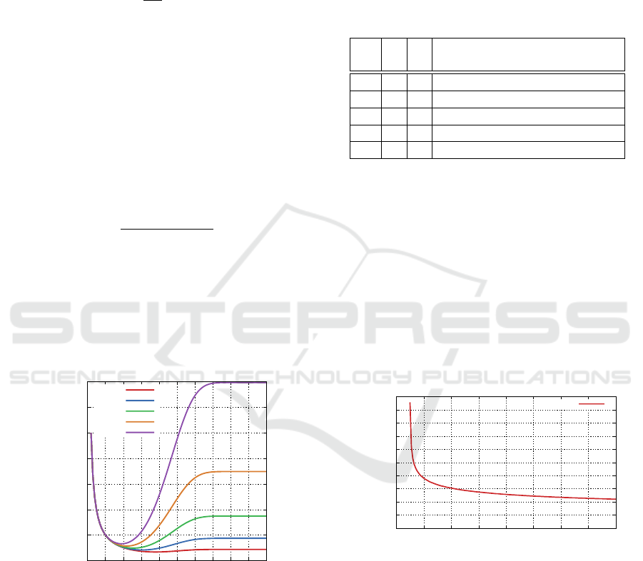
Figure 2: The functions of the relative cost of maintaining
efficiency in the time unit ε
T
for example values of the a
parameter and the Weibull distribution with the parameters
α = β = 5.
It should be noted that in the absence of a finite value
of T , all service replacements are unprofitable. In
such cases, the only economically sensible strategy
is to wait for a failure.
The introduced concepts will be illustrated on an
exemplary Weibull distribution. The Figure 2 shows
the graphs of the ε
T
function for a few example values
of a and the Weibull failure probability
F(t) = 1 − e
−(t/α)
β
, (6)
with the following parameters: α = β = 5. It can be
Table 1: Replacement times that minimize the relative cost
of maintaining the device in service for the specified values
of a and the Weibull distribution of α = β = 5.
a α β Replacement time
to minimize maintenance costs
2 5 5 3.80
4 5 5 3.05
8 5 5 2.57
16 5 5 2.21
32 5 5 1.91
seen from these graphs that the function of the relative
cost of maintaining efficiency takes its minimum the
sooner the higher the value of the a coefficient. This
is in line with the intuition that the higher the cost of
failure compared to the cost of service replacement,
the shorter the time should be the component used. If
the cost of removing the failure is twice as much as the
cost of servicing, the element should be replaced after
3.8 units of time. When the cost of removing a failure
exceeds four times the cost of regular service, the ele-
ment should be replaced after 3.05 time units. A sum-
mary of all values for the above-mentioned graph is
given in the Table 1.
0
1
2
3
4
5
6
7
8
9
10
0 2 4 6 8 10 12 14 16
Service replacement period T
minimizing the cost ε
T
Breakdown cost to service cost ratio a = c
F
/ c
M
min(ε
T
)
Figure 3: Values of T minimizing the relative cost of main-
taining efficiency in the time unit ε
T
for the given values of
the parameter a.
Figure 3 shows how the maximum lifetime of
a given component changes if the relative cost of
failure increases. The presented ones concerned the
Weibull distribution with the parameters α = β = 5. If
the aging process of a given element is approximated
by the Weibull distribution with different values of
these parameters, then the entire analysis should be
performed again for the modified data.
ICEIS 2022 - 24th International Conference on Enterprise Information Systems
366

3 EXAMPLES OF
OPTIMISATION FOR REAL
INDUSTRIAL ELEMENTS
For the purposes of this article, certain parts have been
selected. They are: membrane, swivel joint, bando
belt and IR belt. This parts are shown in Figure 4.
a) Membrane b) Swivel joint
c) Bando belt d) IR belt
Figure 4: Industrial spare parts used as examples for main-
tenance cost optimisation.
The data on the failure-free operation time of individ-
ual spare parts can be found in the Table 2.
Table 2: Uptime in days for each industrial spare part.
Spare part Uptime (days)
Membrane 1, 40, 45, 16, 6, 29, 6, 76, 14,
34, 58, 91, 49, 42, 156, 28, 35,
88, 96, 106, 13, 17
Swivel joint 72, 208, 51, 153, 245, 119, 41,
692, 79, 235, 99, 342
Bando belt 14, 55, 107, 44, 146, 63, 18,
78, 42, 41, 40, 28, 59, 7, 106,
48, 24, 66, 23, 50, 3, 67, 7, 43,
72, 1, 75, 37, 27, 49, 34, 49, 6,
74, 91
IR belt 130, 373, 172, 178, 272, 138,
303, 85
They were used to determine the parameters for the
Weibull distribution using the variable linearization
method and the least squares method (Lai et al.,
2006), (Lai, 2014). The approximation results were
illustrated with probability graphs for each of the an-
alyzed spare parts.
# Import libraries.
from reliability.Distributions import \
Weibull_Distribution
from reliability.Fitters import Fit_Weibull_2P
import matplotlib.pyplot as plt
# Set uptime data.
data = [85,130,138,172,178,272,303,373]
# Prepare Probability Plot using least
# square method. It also determine Weibull
# distribution parameters.
fit = Fit_Weibull_2P(failures=data, \
method=’LS’, linewidth=2.5)
# To get details about determined distribution
# use properties and functions of
# fit.distribution
# object. It is possible to get both plots and
# numeric data.
# ... Add plot options and show ...
plt.show()
In this part, the use of open Python libraries for mod-
eling the life expectancy of exemplary spare parts
used in industry will be presented. For more in-
formation on using Python libraries to analyze and
parameterize the Weibull distribution, see the article
(Chmielowiec and Klich, 2021). The obtained results
will be the basis for determining the optimal operat-
ing times for each part. They can be considered as
the first level to support the parts replacement man-
agement process.
It should be noted that the choice of the Weibull
distribution as a distribution modeling the life cy-
cle of spare parts used in industry is not accidental.
Since the introduction (Weibull, 1939), this distri-
bution is widely used in numerous industrial issues:
strength of glass (Keshevan et al., 1980), pitting cor-
rosion (Sheikh et al., 1990), adhesive wear of met-
als (Queeshi and Sheikh, 1997), failure rate of shells
(Almeida, 1999), failure frequency of brittle materi-
als (Fok et al., 2001), failure rate of composite ma-
terials (Newell et al., 2002), wear of concrete ele-
ments (Li et al., 2003), fatigue life of aluminum alloys
(Hemphill et al., 2012), fatigue life of Al-Si castings
(Aigner et al., 2018), strength of polyethylene tereph-
thalate fibers (Xie et al., 2020), failure of joints under
shear (Bai et al., 2020) or viscosity-temperature rela-
tion for damping fluids (Chmielowiec et al., 2021).
On the basis of financial data, the optimal times
for replacing individual elements were also deter-
mined. Although these times optimize the operating
costs of each part separately, they do not allow to look
at the problem from a global point of view – there
are hundreds of such elements functioning in a man-
ufacturing company. Therefore, in the next the use of
rectangular knapsack problem algorithms to support
the management process of maintenance costs will be
discussed.
Global Spare Parts Exploitation Costs Optymization and Its Reduction to Rectangular Knapsack Problem
367
3.1 Membrane
The membrane is one of the key components of the
pneumatic valve actuator, which is used to create
a vacuum in an electric press. The press and the valve
mounted in it operate in cycles of approximately 20
seconds. During this time, the membrane is subjected
to forces causing its systematic wear. A rupture in
the membrane causes the production line to stop com-
pletely for τ
1
= 4 h. The cost of replacing an element
is C
M,1
= 200 EUR, and the cost of stopping a line is
approximately C
D,1
= 650 EUR h. Therefore, the cost
of an emergency replacement of this element should
be estimated at C
F,1
= C
M,1
+ τ
1
C
D,1
= 2 800 EUR.
This means the a ratio for the membrane is 14.0.
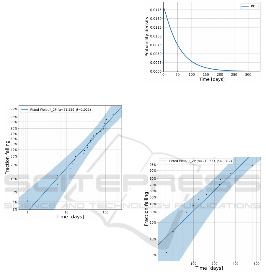
Figure 5: Membrane Weibull probability plot determined
by coordinate linearization and less square method.
Using the data on the failure rate of the element,
it is possible to estimate the parameters of the dis-
tribution. The Figure 5 shows the method of deter-
mining the parameters using the least squares method.
The parameters obtained by this way have the value
α
1
= 51.559 and β
1
= 1.021. The Weibull distribu-
tion density plot for such parameters is presented in
Figure 6. Determining the optimal replacement time
as a value that minimizes the ε
T
function given by
the equation (5), we get T
1
= 980 days. Observing
the historical data, it can be concluded that in practice
it means replacement only in the event of a failure.
This is due to the fact that the β parameter value for
the membrane is very close to 1, and for this value,
preventive replacements are unprofitable at all (Naka-
gawa, 2003).
Figure 6: Membrane Weibull PDF for α = 51.559 and β =
1.021.
3.2 Swivel Joint on an Industrial Robot
The swivel joint is an element installed on the head
of an industrial robot that applies a seal to the
car window. It connects the material feeding hose
(polyurethane mass) with the movable robot head.
The tool on which the swivel is installed travels
Figure 7: Swivel joint Weibull probability plot determined
by coordinate linearization and less square method.
around the three edges of the glass approximately ev-
ery 70 seconds. During this time, the joint rotates 270
degrees and returns to the zero position at the end of
the robot cycle. Swivel joint wear occurs as a result
of repeated rotation, and its sign is loss of tightness or
blockage of movement. Damage of the swivel causes
the production line to stop completely for τ
2
= 1 h.
The cost of replacing it is C
M,2
= 60 EUR, and the
cost of stopping the line is the same as membrane, ap-
proximately C
D,2
= 650 EUR h. Therefore, the cost
of an emergency replacement for this item should be
ICEIS 2022 - 24th International Conference on Enterprise Information Systems
368
estimated at C
F,2
= C
M,2
+ τ
2
C
D,2
= 710 EUR. This
means the a factor for a swivel joint is 11.833.
Using the data on the failure rate of the swivel
joint, it is possible to estimate the parameters of the
distribution. The Figure 7 shows the process of deter-
mining the parameters using the least squares method.
The parameters calculated with this method have the
value α
2
= 210.551 and β
2
= 1.317. The Weibull dis-
tribution density plot for the determined parameters
is presented in Figure 8. Determining the optimal re-
Figure 8: Swivel joint Weibull PDF for α = 210.551 and
β = 1.317.
placement time for this item, we get T
2
= 87 days.
After this time, the swivel joint should therefore be
serviced.
3.3 Bando Belt
Bando belt is an element that transports glass waste
after the breaking operation. It works in a fast cy-
cle, every 16 seconds, starting and braking with great
torque. The belt works at ambient temperature and is
exposed to high tensile forces. The symptom of fail-
ure is partial or complete breaking of the belt. Dam-
age to the Bando belt causes a complete production
line stop at τ
3
= 4 h. The cost of replacing it is
C
M,3
= 1 000 EUR, and the cost of stopping the line
is the same as the memabrane and the swivel, approx-
imately C
D,3
= 650 EUR h. Therefore, the cost of an
emergency replacement of this element should be es-
timated at C
F,3
= C
M,3
+ τ
3
C
D,3
= 3 600 EUR. This
means that the a ratio for a Bando belt is 3.6.
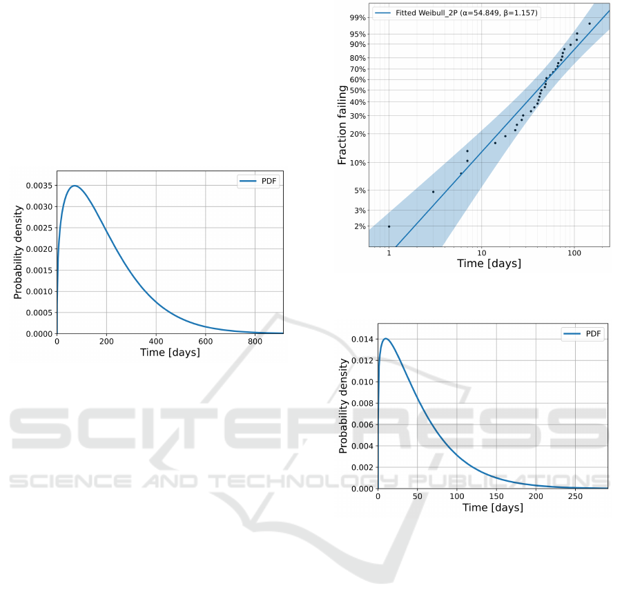
Using the Bando belt failure rate data it is possi-
ble to estimate distribution parameters. The Figure
9 shows the process of determining the parameters
using the least squares method. The parameters ob-
tained with this method have the value α
3
= 54.849
and β
3
= 1.157. The Weibull distribution density plot
for the determined parameters is presented in Figure
10. Determining the optimal replacement time for this
Figure 9: Bando belt Weibull probability plot determined
by coordinate linearization and less square method.
Figure 10: Bando belt Weibull PDF for α = 54.849 and
β = 1.157.
item, we get T
3
= 237 days. After this time, the Bando
belt should be serviced.
3.4 IR Belt
The IR belt is a transport mesh that transports the
glass through the paint drying zone after the screen
printing process. The belt works with constant dy-
namics (speed and acceleration), but in an environ-
ment of increased temperature - 180 degrees Celsius.
Belt failure usually manifests as belt stretching be-
yond the adjustment value (critical length) or break-
ing completely. Damage to the IR belt causes the pro-
duction line to stop completely for τ
4
= 8 h. The cost
of replacing it is C
M,4
= 5 200 EUR, and the cost of
stopping the line is the same as for all other elements,
and is approximately C
D,4
= 650 EUR h. Therefore,
the cost of an emergency replacement of this ele-
ment should be estimated at C
F,4
= C
M,4
+ τ
4
C
D,4
=
Global Spare Parts Exploitation Costs Optymization and Its Reduction to Rectangular Knapsack Problem
369
10 400 EUR. This means that the a ratio for a Bando
belt is 2.0.
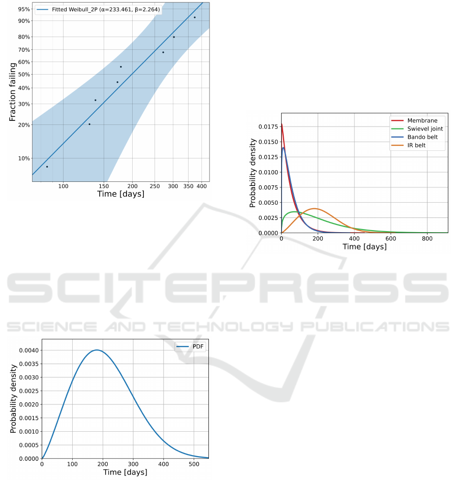
Figure 11: IR belt Weibull probability plot determined by
coordinate linearization and less square method.
Using the IR belt failure rate data it is possible
to estimate distribution parameters. The Figure 11
shows the process of determining the parameters us-
ing the least squares method. The parameters ob-
tained by this method have the value α
4
= 233.461
and β
4
= 2.264. The Weibull distribution density plot
for the determined parameters is presented in Figure
12. Determining the optimal replacement time for this
Figure 12: IR belt Weibull PDF for α = 233.461 and β =
2.264.
item, we get T
4
= 222 days. After this time, service
replacement of the IR belt should take place.
4 REDUCTION OF THE
OPTIMIZATION COST
PROBLEM FOR MULTIPLE
PARTS TO A RECTANGULAR
KNAPSACK PROBLEM
The examples presented in the previous section
clearly show that the optimal replacement times vary
greatly between the different parts, as it is shown in
Figure 13. Therefore, it becomes practically impossi-
Figure 13: Common Weibull PDF plot for all presented
parts.
ble to optimize the replacement time for all elements,
which may be even several hundred in the enterprise.
However, the question arises whether the downtime
caused by a failure cannot be used to replace other
parts as well, and not only the damaged one. Com-
puter aided calculations can estimate the profitability
of immediate replacement of every spare part operat-
ing in the factory. Thus, the IT system may propose
preventive replacement of other parts to the mainte-
nance department at the time of failure. The effect of
using this type of approach will be the reduction of
the total emergency downtime of the line, which will
contribute to the reduction of maintenance costs in the
enterprise.
The presented proposal is a definitely new ap-
proach to the problem of optimization of operating
costs in an enterprise. The classical methods are lim-
ited to the use of analytical methods of the probability
theory and reliability theory. This article presents the
global optimization method, which combines analyti-
cal and discrete methods. The cost reduction method
presented here is one of many possible approaches
to optimizing the performance of maintenance teams.
However, it fits perfectly into modern trends in predic-
tive maintenance for the needs of large-scale produc-
tion of automotive industry companies. It also opens
up wide possibilities of using machine learning mech-
ICEIS 2022 - 24th International Conference on Enterprise Information Systems
370
anisms to better estimate the failure rate function F(t)
and to determine global minima for the operating cost
function.
In order to create an algorithm to support the
decision-making process in the maintenance system,
it is necessary to define a common measure that de-
termines the condition of the production line. Such
a measure will be the expected cost of keeping the line
operational from now until the next planned down-
time. Suppose the line uses n spares U
1
,U
2
,...,U
n
.
Each of the U
i
parts has a set of parameters that de-
fine it. It can therefore be said that
U
i
= (t
i
,α
i
,β
i
,F
i
,G
i
,µ
i
(t),C
M,i
,C
D,i
,τ
i
,σ
i
), (7)
where t
i
is the current time of failure-free operation of
the element, α
i
,β
i
are the Weibull distribution param-
eters defining the failure rate of F
i
and the reliability
of G
i
, µ
i
(t) is the expected uptime of the element after
working t time units, C
M,i
is the cost of component re-
placement during planned downtime, C
D,i
is the cost
of production line downtime, τ
i
is the downtime re-
quired to replace the component, and σ
i
is the part of
the human resources that is used during the replace-
ment of a given item. If it is assumed that the next
scheduled stoppage will take place for T units of time,
then the expected cost of operating a part of U
i
at that
time is
C(U
i
,T ) =
¯
k
i
C
F,i
+ G
i
(t
0
i
)C
M,i
, (8)
where C
F,i
= C
M,i
+τ
i
C
D,i
is the cost of an emergency
replacement part,
¯
k
i
= 1 + k
i
+ F
i
(t
0
i
) is the expected
number of failures in time to the scheduled downtime,
and G
i
(t
0
i
) is the probability of failure-free operation
of the part from the time of the last forecast failure
to the scheduled downtime. The expected number of
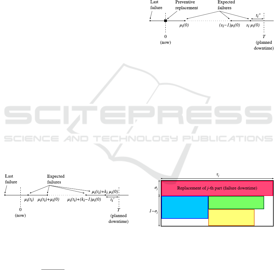
Figure 14: Expected failures in the case of not carry out
preventive replacement of the element.
failures can be obtained by assuming the following
values for k
i
and t
0
i
k
i
=
T − µ
i
(t
i
)
µ
i
(0)
, (9)
t
0
i
= min (T − µ
i
(t
i
) − k
i
µ
i
(0),T ) . (10)
Note that if T < µ
i
(t
i
), then k
i
= −1 and the expected
number of failures is
¯
k
i
= F
i
(T ). The interpretation of
k
i
and t
0
i
is shown in Figure 14.
Additionally, we define the alternative expected
cost of operating the U
i
part
C
0
(U
i
,T ) = ¯s
i
C
F,i
+ (1 + G
i
(t
00
i
))C
M,i
, (11)
for which ¯s
i
= s
i
+ F
i
(t
00
i
), s
i
= bT /µ
i
(0)c and t
00
i
=
T − s
i
µ
i
(0). This function expresses the expected al-
ternative costs that will be incurred in the event that
part of U
i
has been replaced at present on the occa-
sion of downtime due to failure of another part. The
interpretation of s
i
and t
00
i
is shown in Figure 15.
Figure 15: Expected failures in the event of a preventive
replacement of an element.
For the functions C and C
0
defined in this way, we
create a sequence of values V
i
= C(U
i
,T ) −C
0
(U
i
,T ),
which express the expected profit on the replacement
of U
i
during the emergency downtime. If we assume
that the part with index j failed, then the optimization
problem can be reduced to a two-dimensional knap-
sack problem. It should be assumed that the knapsack
has the shape of a rectangle with a width of τ
j
and
a height of 1 − σ
j
, and the elements arranged in it are
rectangles of width τ
i
, height σ
i
and values V
i
, where
i 6= j. It should also be emphasized that the elements
placed in the knapsack cannot be twisted, as time and
human resources are not interchangeable. Figure 16
illustrates the problem described above.
Figure 16: Optimum use of downtime for the preventive
replacement of additional parts.
The literature devoted to this problem is very
rich. The best review article to date is (Neuenfeldt Jr.
et al., 2022). During a systematic review of bibli-
ographic items, the authors distinguished four basic
approaches to the construction of algorithms for solv-
ing the two-dimensional rectangular knapsack prob-
lem: approximation, exact, heuristic and hybrid. The
article presents a very in-depth bibliometric analysis
indicating which publications have the most signifi-
Global Spare Parts Exploitation Costs Optymization and Its Reduction to Rectangular Knapsack Problem
371

cant impact on the development of algorithms solv-
ing this problem. The review includes over one hun-
dred publications issued by 2020. The intensity of
research in this area is also evidenced by numerous
publications issued in the last two years: (Zhou et al.,
2019), (Fırat and Alpaslan, 2020), (Wei et al., 2020),
(Li et al., 2021) and (Wang et al., 2021b).
5 CONCLUSIONS
The article presents how the methods of analytical
and discrete optimization can be used to minimize the
operating costs of a production line. The third part
presents analytical methods of cost optimization for
a single spare part. The MES (Manufacturing Ex-
ecution System) equipped with this type of mecha-
nisms can keep the maintenance manager informed
about the probability of failure of a given part and the
expected costs of its removal. It provides the cur-
rent knowledge of what events should be prepared
for and what to expect in the near future. On the
other hand, the equations (8) and (11) introduced in
the fourth part constitute the basis for estimating the
actual value of the service activity. The algorithm
of conduct presented in this section is to support the
decision-making process in the area of maintenance
from the perspective of the entire enterprise. The
complexity of the two-dimensional knapsack problem
indicates that the global optimization problem is ex-
tremely computationally difficult. Therefore, the ac-
tual functioning of global methods of minimizing op-
erating costs in real time requires significant comput-
ing power. Therefore, the presented approach requires
further research in the field of, for example, simplifi-
cation of the model, which will result in a reduction
of computational complexity.
Nevertheless, the use of heuristic methods, which
relatively quickly indicate the first approximation of
the solution to the problem, will be appropriate in
this case. We should remember that the system is
supposed to support decision-making, and not com-
pletely eliminate the human factor. Therefore, even
suggestions of possible solutions will give very valu-
able information for the maintenance manager and
can be successfully used in modern MES systems.
REFERENCES
Aigner, R., Leitner, M., and Stoschka, M. (2018). Fatigue
strength characterization of al-si cast material incor-
porating statistical size effect. In Henaff, G., edi-
tor, 12th International Fatigue Congress (FATIGUE
2018), volume 165 of MATEC Web of Conferences.
Almeida, J. (1999). Application of weilbull statistics to the
failure of coatings. Journal of Materials Processing
Technology, 93:257–263.
Ansell, J., Bendell, A., and Humble, S. (1984). Age re-
placement under alternative cost criteria. Management
Science, 30(3):358–367.
Bai, Y.-L., Yan, Z.-W., Ozbakkaloglu, T., Han, Q., Dai,
J.-G., and Zhu, D.-J. (2020). Quasi-static and dy-
namic tensile properties of large-rupture-strain (LRS)
polyethylene terephthalate fiber bundle. Construction
and Building Materials, 232.
Barlow, R. and Proschan, F. (1965). Mathematical theory
of reliability. John Wiley & Sons, New York.
Barlow, R. and Proschan, F. (1975). Statisitcal Theory of
Reliability and Life Testing. Holt, Rinehart, Austin.
Berg, M. and Epstein, B. (1978). Comparison of age, block,
and failure replacement policies. IEEE transactions
on Reliability, 27(1):25–29.
Chmielowiec, A. and Klich, L. (2021). Application of
python libraries for variance, normal distribution and
Weibull distribution analysis in diagnosing and op-
erating production systems. Diagnostyka, 22(4):89–
105.
Chmielowiec, A., Wo
´
s, W., and Gumieniak, J. (2021). Vis-
cosity Approximation of PDMS Using Weibull Func-
tion. Materials, 14(20):6060.
Christer, A. (1978). Refined asymptotic costs for renewal
reward processes. Journal of the Operational Re-
search Society, 29(6):577–583.
Cl
´
eroux, R., Dubuc, S., and Tilquin, C. (1979). The age
replacement problem with minimal repair and random
repair costs. Operations Research, 27(6):1158–1167.
Cl
´
eroux, R. and Hanscom, M. (1974). Age Replacement
With Adjustment and Depreciation Costs and Interest
Charge. Technometrics, 16(2):235–239.
Finkelstein, M., Cha, J., and Levitin, G. (2020). On
a new age-replacement policy for items with observed
stochastic degradation. Quality and Reliability Engi-
neering International, 36(3):1132–1143.
Fırat, H. and Alpaslan, N. (2020). An effective approach to
the two-dimensional rectangular packing problem in
the manufacturing industry. Computers & Industrial
Engineering, 148:106687.
Fok, S., Mitchell, B., Smart, J., and Marsden, B. (2001).
A numerical study on the application of the weibull
theory to brittle materials. Engineering Fracture Me-
chanics, 68:1171–1179.
Fox, B. (1966). Letter to the Editor – Age Replacement with
Discounting. Operations Research, 14(3):533–537.
Frees, E. and Ruppert, D. (1985). Sequential nonparamet-
ric age replacement policies. The Annals of Statistics,
13(2):650–662.
Fu, Y., Yuan, T., and Zhu, X. (2018). Optimum pe-
riodic component reallocation and system replace-
ment maintenance. IEEE transactions on reliability,
68(2):753–763.
Glasser, G. (1967). The age replacement problem. Techno-
metrics, 9(1):83–91.
ICEIS 2022 - 24th International Conference on Enterprise Information Systems
372

Hemphill, M., Yuan, T., Wang, G., Yeh, J., Tsai, C.,
Chuang, A., and Liaw, P. (2012). Fatigue behavior of
al0.5cocrcufeni high entropy alloys. Acta Materialia,
60(16):5723–5734.
Ingram, C. and Scheaffer, R. (1976). On consistent esti-
mation of age replacement intervals. Technometrics,
18(2):213–219.
Keshevan, K., Sargent, G., and Conrad, H. (1980). Sta-
tistical analysis of the hertzian fracture of pyrex glass
using the weibull distribution function. Journal of Ma-
terials Science, 15:839–844.
Knopik, L. and Migawa, K. (2017). Optimal age-
replacement policy for non-repairable technical ob-
jects with warranty. Eksploatacja i Niezawodnosc -
Maintenance and Reliability, 19(2):172–178.
Lai, C. (2014). Generalized Weibull Distributions. Springer,
Heidelberg.
Lai, C., Murthy, D., and Xie, M. (2006). Weibull distri-
butions and their applications. In Pham, H., editor,
Springer Handbook of Engineering Statistics, pages
63–78. Springer London, London.
L
´
eger, C. and Cl
´
eroux, R. (1992). Nonparametric age re-
placement: bootstrap confidence intervals for the op-
timal cost. Operations research, 40(6):1062–1073.
Li, Q., Fang, J., Liu, D., and Tang, J. (2003). Failure proba-
bility prediction of concrete components. Cement and
Concrete Research, 33:1631–1636.
Li, Y.-B., Sang, H.-B., Xiong, X., and Li, Y.-R. (2021).
An improved adaptive genetic algorithm for two-
dimensional rectangular packing problem. Applied
Sciences, 11(1):413.
Nakagawa, T. (2003). Maintenance and optimum policy. In
Pham, H., editor, Handbook of reliability engineering,
pages 367–395. Springer.
Nakagawa, T. (2006). Statistical models on maintenance. In
Pham, H., editor, Springer Handbook of Engineering
Statistics, pages 835–848. Springer London, London.
Neuenfeldt Jr., A., Silva, E., Francescatto, M., Rosa, C.,
and Siluk, J. (2022). The rectangular two-dimensional
strip packing problem real-life practical constraints:
A bibliometric overview. Computers & Operations
Research, 137:105521.
Newell, J., Kurzeja, T., Spence, M., and Lynch, M. (2002).
Analysis of recoil compressive failure in high perfor-
mance polymers using two-, four-parameter weibull
models. High Performance Polymers, 14:425–434.
Queeshi, F. and Sheikh, A. (1997). Probabilistic characteri-
zation of adhesive wear in metals. IEEE Transactions
on Reliability, 46:38–44.
Ran, A. and Rosenlund, S. (1976). Age replacement with
discounting for a continuous maintenance cost model.
Technometrics, 18(4):459–465.
Scmeaffer, R. (1971). Optimum Age Replacement Poli-
cies with an Ikreasing Cost Factor. Technometrics,
13(1):139–144.
Sheikh, A., Boah, J., and Hansen, D. (1990). Statistical
modelling of pitting corrosion and pipeline reliability.
Corrosion, 46:190–196.
Subramanian, R. and Wolff, M. (1976). Age replacement in
simple systems with increasing loss functions. IEEE
Transactions on Reliability, 25(1):32–34.
Wang, J., Qiu, Q., and Wang, H. (2021a). Joint optimization
of condition-based and age-based replacement policy
and inventory policy for a two-unit series system. Re-
liability Engineering and System Safety, 205:107251.
Wang, T., Hu, Q., and Lim, A. (2021b). An exact algorithm
for two-dimensional vector packing problem with vol-
umetric weight and general costs. European Journal
of Operational Research.
Wei, L., Lai, M., Lim, A., and Hu, Q. (2020). A branch-and-
price algorithm for the two-dimensional vector pack-
ing problem. European Journal of Operational Re-
search, 281(1):25–35.
Weibull, W. (1939). A statistical theory of the strength of
material. Ingeniors Vetenskaps Akademiens Handli-
gar, 151:5–45.
Xie, S., Lin, H., Wang, Y., Chen, Y., Xiong, W., Zhao,
Y., and Du, S. (2020). A statistical damage consti-
tutive model considering whole joint shear deforma-
tion. International Journal of Damage Mechanics,
29(6):988–1008.
Zhao, X., Al-Khalifa, K., Hamouda, A., and Nakagawa, T.
(2017). Age replacement models: A summary with
new perspectives and methods. Reliability Engineer-
ing & System Safety, 161:95–105.
Zhao, X., Li, B., Mizutani, S., and Nakagawa, T. (2021).
A Revisit of Age-Based Replacement Models With
Exponential Failure Distributions. IEEE Transactions
on Reliability.
Zhou, S., Li, X., Zhang, K., and Du, N. (2019). Two-
dimensional knapsack-block packing problem. Ap-
plied Mathematical Modelling, 73:1–18.
Global Spare Parts Exploitation Costs Optymization and Its Reduction to Rectangular Knapsack Problem
373
