
Assessment of Dose Reduction Strategies in Wavelength-selective
Neutron Tomography
Victoria H. DiStefano, Jacob M. LaManna, David L. Jacobson, Paul A. Kienzle, Daniel S. Hussey
and Peter Bajcsy
National Institute of Standards and Technology, Gaithersburg, MD 20899, U.S.A.
Keywords: 3D Reconstruction Image Quality, Dose Reduction, Neutron Imaging.
Abstract: The goal of this study is to determine variable relationships and a computational workflow that yield the
highest quality of three-dimensional reconstructions in neutron imaging applications with reduced number of
projections angles. Neutrons interact with matter primarily through the strong nuclear force providing unique
image contrast modes. Accessing many of these contrast modes requires defining the energy of the neutron
beam, resulting in long exposure times for a single two-dimensional projection image. To collect of order
100 tomograms at different neutron wavelengths within a reasonable time frame (less than 1 week) suggests
the use of dose reduction tomography reconstruction algorithms. We identified and evaluated the main factors
affecting the quality of the 3D tomographic reconstruction in the computational image workflow: the
projection number, the reconstruction method, and the post-processing method. This study reports several
relationships between 3D reconstruction quality metrics and acquisition time. Based on the established
relationships, the performance of a seeded simultaneous iterative reconstruction technique (SIRT) yielded
improved image quality and more accurate estimates of the reconstructed attenuation values compared to a
SIRT without a priori information or a trained neural network based on a mixed scale dense network.
1 INTRODUCTION
The properties of the neutron, a massive, neutral spin-
1/2 particle that interacts primarily through the strong
nuclear force, enable one to create images with
unique sources of contrast compared to other
penetrating probes. From the de Broglie relationship,
a massive particle can be thought of as a wave, whose
wavelength is inversely related to its kinetic energy
(Rauch & Werner, 2015). The diverse set of neutron
image contrasts include quantitative imaging of
magnetic and electric fields with polarized neutron
imaging (Hilger et al., 2018; Jau et al., 2020),
characterizing the porosity with sub-pixel resolution
through dark-field or phase imaging (Brooks et al.,
2017; Strobl, 2014), and crystal phase mapping with
Bragg-edge imaging (Vitucci et al., 2018; Woracek et
al., 2014). Common to these sources of image
contrast is the need to define the neutron wavelength
and to acquire image data sets at many (on order of
100) different instrument settings, which we refer to
as a scan parameter. Several of these scan parameters
contribute to extended neutron image acquisition
times which affect image quality and measurement
throughput of samples under scientific investigations.
Neutron sources are already about 1 billion times less
intense than synchrotron X-ray sources. The need to
define the neutron energy in monochromatic beams
results in a factor of 10 to 1000 loss in neutron fluence
rate compared to the full polychromatic beam. Thus,
the exposure time for a single two-dimensional image
is on the order of 1 minute. To acquire 100
tomograms with reasonable experimental
measurement time (beam time at a user facility is
typically about 1 week) thus requires one to sacrifice
spatial resolution, temporal resolution, wavelength
resolution and/or acquiring a reduced number of
angular projections. This work is motivated by
minimizing the acquisition time while maximizing
the quality of 3D tomographic reconstructions.
Another common feature of the wavelength-
selective image contrasts is that the image contrast
varies somewhat slowly for each successive scan
parameter setting. We postulate that it will be
possible to obtain quantitative multiscale data by
proper choice of a dose reduction tomography
reconstruction algorithm using a priori data from a
66
DiStefano, V., LaManna, J., Jacobson, D., Kienzle, P., Hussey, D. and Bajcsy, P.
Assessment of Dose Reduction Strategies in Wavelength-selective Neutron Tomography.
DOI: 10.5220/0011077600003209
In Proceedings of the 2nd International Conference on Image Processing and Vision Engineering (IMPROVE 2022), pages 66-77
ISBN: 978-989-758-563-0; ISSN: 2795-4943
Copyright
c
2022 by SCITEPRESS – Science and Technology Publications, Lda. All rights reserved

tomography data set with sufficient angular
projections (that is, the outer edge of the object
traverses about one pixel for a rotation step). To test
this, we will use Bragg-edge imaging to identify the
crystal phases in samples of well-known
composition. There are many dose reduction
algorithms in the literature, as a first step we have
chosen to compare the simultaneous iterative
reconstruction technique (SIRT) as implemented in
the ASTRA Toolbox (Palenstijn et al., 2011b; Van
Aarle et al., 2015a; van Aarle et al., 2016) and a
machine learning algorithm that uses a trained mixed
scale dense convolutional neural network (MS-D)
(Pelt & Sethian, 2017). Our goal is to establish
models and rankings among the factors that affect 3D
reconstruction image quality and acquisition time in
order to guide neutron imaging experimentalists in
maximizing image quality and minimizing
acquisition time. Our approach is to design a
metrology for quantifying the trade-offs between
several image quality metrics and different dose
reduction approaches (acquisition time reduction).
In our experimental design, we varied the number
of projections (60, 80, 360, 600, and 800) and a
chosen 3D tomographic reconstruction method
(SIRT, SIRT + seed). For each combination of these
two variables, the MS-D Neural Network (NN)
training was performed as a post-processing step with
the input training sets consisting of 2D frames. First,
accuracy of reconstructed tomographic volumes is
related to the number of acquired 2D projections via
a theoretical relationship (Kak, A. C., Slaney, M., &
Wang, G., 2002). Next, accuracy by the MS-D NN
was measured using the root mean square error
(RMSE) metric between the training low projection
number input and the training high projection number
output (2400). Finally, quality of 3D reconstructions
was measured by 24 blur metrics per image and by
the signal to noise ratio (SNR) per manually
segmented reference object. The combination of
minimum RMSE, optimal blur, and maximum SNR
metrics defines our evaluation framework for
minimizing the imaging acquisition time (i.e.,
proportional to the number of 2D projections) and
maximizing the quality of 3D tomographic
reconstructions.
The Contributions of Our Work Lie in:
(1) a factorial experimental design to understand
trade-offs between acquisition time and image
quality of 3D tomographic reconstructions from
neutron imaging data,
(2) evaluating (a) reference material-based image
quality such as SNR, (b) imaging quality focused
metrics such as blur, (c) reference 3D
reconstruction acquired for oversampled 2D
projections such as RMSE, and (d) theory for
circularly symmetric objects and the relationship
between intensity variance and the number of 2D
projections.
(3) including the MS-D NN model-based denoising
as a postprocessing step to leverage previously
acquired high quality dataset.
The novelty of this work is in establishing model-
based and ranking relationships between 3D
reconstruction accuracy and acquisition time
represented by intensity variance, SNR, RMSE, blur,
number of 2D projections, number of iterations and
seeding of 3D tomographic reconstruction (SIRT), and
supervised postprocessing denoising model (MS-D Net
model). The relationships are summarized in Table 4.
2 RELATED WORK
Related work to our approach can be found in the
literature about 3D tomographic reconstruction
algorithms and about image quality metrics.
3D Tomographic Reconstruction Algorithms: The
two main computed tomography (CT) reconstruction
algorithms that reconstruct the raw 2D projections
into 3D space are Filtered Back Projection and
Iterative Reconstruction. The mathematical theory for
these algorithms are beyond the scope of this work
but are detailed in (Kak et al., 2002). In simple Back
Projection (BP), a slice is reconstructed by ‘smearing
out’ the line integrals for each angle and summing
them together. The Filtered Back Projection (FBP)
corrects this process by applying a spatial frequency
filter to account for the oversampling in certain areas
(Schofield et al., 2020).
In recent years, improvements in computer
processing have made Iterative Reconstruction (IR)
techniques popular for dose and noise reduction.
There are several types of IR algorithms, but the most
complex algorithms forward-project a reconstruction
image (either initialized with a blank image or a
reconstruction image) and creates a simulated
sinogram (Tayal et al., 2019). The simulated
sinogram is then compared to the sinogram of the raw
data and corrections to the reconstruction image are
made. The algorithm iterates through this process a
set number of times. In the SIRT, the projection
differences and sinogram differences are weighted.
Additional details can be found in (Kak et al., 2002;
Tayal et al., 2019; Van Aarle et al., 2016a). For both
the FBP and SIRT algorithms, the image quality and
accuracy increase with an increasing number of
projections.
Assessment of Dose Reduction Strategies in Wavelength-selective Neutron Tomography
67

Image Quality in 3D Neutron Imaging: The quality
can be assessed after a 3D tomographic
reconstruction is calculated. The quality metrics can
evaluate (a) the reconstruction against a priori known
reconstruction using the root mean square error
(RMSE), (b) foreground vs. background
discrimination using signal-to-noise ratio (SNR) over
calibration regions, (c) optical focus of imaging on an
object of interest in a camera field of view using blur
metrics, and (d) the reconstruction accuracy as a
function of the number of 2D projections following a
theoretical model. Each quality evaluation requires
some assumptions about a priori knowledge. RMSE
assumes co-registered ground truth 3D
reconstruction. SNR quantification requires known
foreground and background masks. Blur metrics are
derived from intensity histograms using multiple
mathematical models that must be empirically
chosen. In our work, the ground truth 3D
reconstruction is established from over-sampled
angular 2D projections (2400 projections). Next,
foreground and background masks are created
manually for two reference cylindrical objects filled
with known material. Finally, an optimal blur
mathematical model is chosen by maximizing blur
coefficient of variation over 24 models and by
including human assessment (Crete et al., 2007a;
Petruccelli et al., n.d.).
3 MATERIALS AND METHODS
Figure 1 shows an overview of the key components
in evaluating the trade-offs between acquisition time
(dose reduction) and 3D reconstruction quality. These
key components hide the relationships among
variables, such as number of 2D projections (or
acquisition time), number of iterations during 3D
reconstruction, variance of intensities in 3D
reconstructed dataset, SNR, RMSE, blur, and
availability of highly accurate seed for a 3D
reconstruction algorithm and supervised
postprocessing model. Following figure 1, this
section describes each component in our assessment
of dose reduction strategies.
Figure 1: An overview of assessing dose reduction
strategies.
3.1 Samples
The test sample set consisted of four geological
samples to analyze. The first two samples were a
meteorite of unknown origin and a 1 cm diameter core
of Westerly Granite, which has been extensively
analyzed in (Bingham et al., 2013; Gates et al., 2018).
The other two samples were standard reference
powders obtained from National Institute of
Standards and Technology (NIST) Standard
Reference Material (SRM) collection. Several grams
of these powders were placed in separate 6061-
aluminum tubes, with 316 stainless steel ferrules
around them, and sealed on both ends with polyimide
tape. The powders were not compacted or leveled off
and aluminum tape was used to secure all the samples
in place. Figure 2A shows an image of the samples
before they were placed in the beam.
The SRM powders were used as reference objects
for all the subsequent metric evaluations. The first
powder, SRM 691 – Reduced Iron Oxide, was an iron
powder consisting of 90 % by mass of iron and trace
amounts of oxides and other metals. The second
powder, SRM 70b – Potassium Feldspar, was
prepared from a high-purity feldspar obtained from
pegmatite deposits in the Black Hills of South
Dakota. The material is a mixture of alkali feldspar,
plagioclase feldspar, quartz, and a small amount of
mica. The SRM was blended and bottled at NIST.
3.2 Beam, Detector and Image
Acquisition
Neutron tomography datasets were measured at the
NG-6 Cold Neutron Imaging Instrument at the NIST
Center for Neutron Research (NCNR) (Hussey et al.,
2015). A dataset with many projection angles was
collected, representing the maximum number of 2D
projections for this study, 2400, evenly spaced over
360 degrees (2399 unique projections). This data set
is referred below as the “high-quality” data set and
serves as ground truth. Figure 2B shows an example
projection image. The dataset was collected using a
polychromic neutron beam that can be approximated
from a kinetic molecular theory as a Maxwell-
Boltzmann distribution with characteristic
temperature of about 50 K (Gavin D. Peckham and
Ian J. McNaught, 1992). An Andor NEO scientific
complementary metal oxide semiconductor (sCMOS)
camera operating in 12-bit mode (Oxford
Instruments, n.d.) was used to collect images from a
P43 scintillator detector (i.e. gadolinium oxysulfide
doped with terbium, Gd2O2S:Tb also known as
GadOx ) with a Nikon Nikkor 50 mm f1.2 lens.
Each image was acquired over 4 seconds and the
median of 5 images was taken for each projection,
IMPROVE 2022 - 2nd International Conference on Image Processing and Vision Engineering
68

leading to maximum intensity around 3500 grey
levels. The pixel pitch of the images was 51.35 µm
(resolution about 100 µm) and the field of view was
2560 pixels by 2160 pixels (~13 cm by 11 cm). This
scan took approximately 16.5 hours to complete.
From this original dataset, several sub-sets were taken
to simulate smaller projection numbers: 60, 80, 360,
600, and 800. Angles from these sets were evenly
taken throughout the 2400 projections in order to span
the same 360-degree sample space. If these datasets
were collected on the beamline, they would take 0.4
hours, 0.6 hours, 2.5 hours, 4.2 hours, and 5.5 hours,
respectively.
Two additional separate datasets using a
monochromatic beam were obtained to validate and
analyze. The first dataset consisted of 720 projections
collected over 360 degrees. Two highly oriented
pyrolytic graphite crystal monochromators were used
to select the wavelength of 0.37 nm and the Δλ/λ was
about 1%. The same camera and lens as above were
used to collect images from a zinc sulfide/lithium
fluoride (ZnS:LiF) scintillator. For this data to be
consistent with the polychromatic datasets in terms of
maximum intensity, the lower incident beam intensity
required each projection image to be acquired over 10
seconds with a median of 3 images (maximum
intensity ~3500 counts). The pixel pitch of the images
was 51.35 µm (resolution about 250 µm) and the field
of view was 2560 pixels by 2160 pixels (about 13 cm
by 11 cm). This scan took approximately 7 hours to
complete. Using this same set up, another scan was
taken with only 80 projections taking approximately
0.8 hours to complete (exposure time is 20 s for the
polychromatic and 30 s for the monochromatic
beam).
Figure 2: Photo of the samples before they were placed in
the beam (A) and a raw neutron projection image (B).
3.3 Computational Workflow
Image Pre-processing: As stated, the images from
each projection angle were combined by taking the
median to remove non-statistical noise such as
gamma streaks and hot spots. An image with the
beam off was used to subtract the additive noise. An
image of the open beam was used to normalize the
projections, and a region of the image that did not
contain a sample was used to correct for any small
drift in beam intensity. The normalized projections
were formed into sinograms, correcting for rotation
axis title. Ring artifacts were removed from the
sinograms by the algorithm developed by Vo et al (Vo
et al., 2018).
Tomographic Reconstruction: We use the SIRT
algorithm, assuming a parallel beam geometry, in the
ASTRA toolbox (Palenstijn et al., 2011b; Van Aarle
et al., 2015a; van Aarle et al., 2016) using the
MATLAB bindings, on a single Nvidia Quadro
RTX5000 GPU card to reconstruct all the of the data
presented (NIST Disclaimer Statement | NIST, n.d.).
The output of the tomography reconstruction is the
average value of the neutron total macroscopic
scattering cross-section, Σ, with units inverse length,
and is analogous to the attenuation coefficient in X-
ray-based measurements.
Image Post-processing: A machine learning post-
processing method was applied to the reconstructions
generated with SIRT. The Mixed-Scale Dense (MS-
D) neural network was trained and validated with
high/low image quality pairs using a Nvidia Quadro
RTX5000 GPU. A total of 5 networks were trained,
varying the low image quality datasets (SIRT60pro,
SIRT80pro, SIRT360pro, SIRT600pro, SIRT800pro)
and using the SIRT2400pro reconstruction for the
high-quality dataset throughout. The MSD net was
run for each network until the root mean square error
(RMSE), computed as the difference from the high-
quality dataset, was below at least 0.00014, taking
anywhere from 1 hour (MS-D Net800) to 288 hours
(MS-D Net80). Each network was then applied to all
the low-quality datasets. We refer to these data as
MS-D NetTT_FFpro, where TT is the number of
projections used to generate the volume used to train
the network, and FF is the number of projections used
to generate the volume that is filtered.
Figure 3 shows an example of the process using
the SIRT-80pro data as the training and validating
dataset (MS-D Net80_80pro).
Assessment of Dose Reduction Strategies in Wavelength-selective Neutron Tomography
69

Figure 3: An example of the MSD-Net Post-Processing
Method using the SIRT 80pro/SIRT 2400pro datasets as
high/low quality pairs (MS-D Net80_80pro). After the
neural network was trained, it was applied to all the low-
quality datasets.
3.4 3D Reconstruction Quality versus
Acquisition Time
Accuracy and Number of 2D Projections: To assess
the accuracy of each reconstruction method as a
function of projection number (aliasing distortions;
Kak, A. C., et. al.., 2002), we evaluated the standard
deviation of the reconstructed values of the SRM
powders, as shown in Figure 5 As discussed in Kak
and Slaney (2002), for a circularly symmetric object,
the variance of the reconstruction is approximated as
varf
0,0=
π
τ
MN
dw
(1)
0,0=
|
|
/
/
(2)
M the number of projections, N
0
the number of
neutrons detected in the center of the object, τ is the
sampling width, and h(t) and its Fourier transform
H(w) the filtering window, which is the ramp function
for the SIRT algorithm used in this work.
SNR and RMSE Metrics: RMSE and SNR metrics
were computed by leveraging reference data cons-
tructed via a tomographic reconstruction from 2400
projections and manual annotation of image regions
delineating standard reference materials in the field of
view – see Figure 4. We calculated RMSE and SNR
using common definitions shown in equations below:
=
∑|
|
(3)
=
̅
(4)
where
is the reference value,
is the measured
value, is the number of values in a tomographic
reconstruction, ̅ is the average intensity and is the
sample standard deviation.
Blur Metrics: Blur mostly affects structure and detail,
which are absent in the reference powders. For this
reason, the blur metrics were analyzed for the whole
image over the entire volume, including the meteorite
and granite. To determine the optimal blur metric for
our datasets, we evaluated 24 different blur/focus
metrics from (Crete et al., 2007a; Petruccelli et al.,
n.d.). We evaluated the metrics based on two
different assumptions: (1) that the optimal metric had
the highest coefficient of variation over a set of
diverse image qualities and (2) that the optimal metric
is one that is verified by a human quality assessment.
For Assumption 1, we investigated if the optimal blur
metric selection was dependent on the dataset
analyzed. We then compared the metrics determined
for each assumption to determine if they ranked
datasets in the same order. For Assumption 2, we used
the no-reference perceptual blur metric developed by
Crete et al., henceforth referred to as the CRETE
method, which has been validated with a human
perception test (Crete et al., 2007a), for which, the
higher the blur metric is, the poorer the visual quality
of the image.
4 EXPERIMENTAL RESULTS
To compare the under-sampled data sets with ground
truth (2400 projections), we took samples at a regular
interval from the polychromatic data set to form data
sets with 60, 80, 360, 600, and 800 projections, we
also refer to these data sets as “low-quality”. From
each of these under-sampled data sets we computed
two reconstructed volumes. We formed the SIRT
estimate of the volume using no prior estimate, and
Figure 4: Left - A cross-section of the reference powders
with the mask overlain on top. The powder regions are
labeled. Right – A cross section of 3D tomographic
reconstruction from 2400 projections which was considered
as a reference.
IMPROVE 2022 - 2nd International Conference on Image Processing and Vision Engineering
70
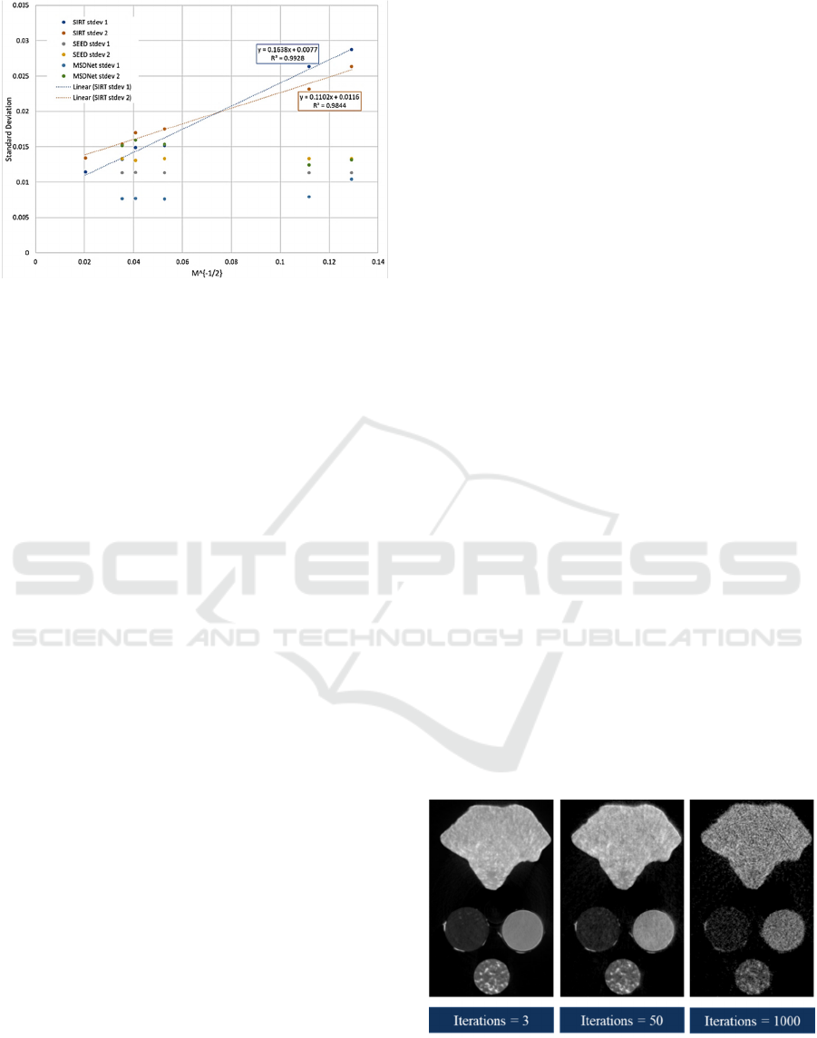
Figure 5: Observed standard deviation for the two
cylindrical regions of interest (SRMs denoted as 1 and 2)
and reconstruction method as a function of number of
projections M. To highlight the linear relationship of the
SIRT data set, the standard deviation is plotted as M
-1/2
In
contrast to SIRT data sets, the SEED and MS-D Net data
sets show approximately constant standard deviations as a
function of M.
we designate these as SIRT-Xpro (where X = 60, 80,
360, 600, 800, or 2400). The second set of volumes
seed the SIRT with a prior estimate from the highly-
quality (SIRT-2400pro) reconstruction, and we
designate these as SIRT+seed-Zpro (where Z = 60,
80, 360, 600 or 800). The 2400 projection dataset was
used to determine the best approaches to evaluate the
metrics for image quality. In addition, we created a
validation dataset reconstructed using the SIRT
function in the ASTRA toolbox from 720 projections
acquired using a monochromatic beam and by using
500 iterations (Palenstijn et al., 2011a; Van Aarle et
al., 2015b, 2016b).
4.1 3D Reconstruction Time
Reconstruction of the 2400 projection dataset took
about 15 hours, while reconstruction of only 80
projections took 0.7 hours. Time to reconstruct an
example volume using the SIRT + seed
reconstruction method Time
Rec
as a function of the
SIRT iterations was linear with the model parameters
in Equation below.
Time
Rec
[s] = 2.1089 [s] * x + 131.85 [s] (5)
where x is the number of SIRT iterations. Here the
SIRT 2400pro dataset was used as a seed and the 80
projection, 3.7 Å monochromatic dataset was
reconstructed. The impact on image quality is
discussed below, however we note that for when using
a prior estimate, only 3 iterations were required to
achieve significant image clarity, and larger number of
iterations exhibited the well-known behavior of over-
fitting of the noise (Chen et al., 2016).
4.2 Acquisition Time and Estimated
Accuracy of 3D Reconstruction
Acquisition time is directly proportional to the
number of acquired 2D projections M. Following the
Equations (1) and (2), the number of 2D projections
M influence the value of N
0
, the number of neutrons.
This is shown in Figure 5 by different slopes and
intercept of the fit of the standard deviation as a
function of M
-1/2
. The standard deviation for the
seeded and MSD-Net reconstructions do not possess
the standard deviation dependence on projection
number, but instead are approximately that of the
SIRT-2400pro data set, which is used as the seed or
ground truth -see Figure 5. The slightly suppressed
standard deviation for the MS-D Net data sets
indicates there is strong smoothing occurring. For the
SIRT+seed data, the a priori information, which is in
part derived from the projections used in the under-
sampled data, reduces the overall variance.
4.3 SNR and RMSE based
Comparisons
For the SNR evaluations, we isolated the standard
reference powders to try and determine if there was a
relationship between the average SNR and the
projection number as a function of the reference
powder regions (SNR=f(region, projection)).
Isolation was realized by manually establishing a 2D
mask in the SIRT-2400pro dataset that defined the
reference powders for each 2D cross-sectional z-
frame and then determined the frame z-range that
corresponded to the reference powders. We then
computed the SNR for each reference powder per z-
frame. We could then rank the datasets based on their
average SNR values and try to determine the
predictive relationship among the data.
Figure 6: Reconstructed slices using 3, 50, and 1000
iterations. Visual quality decreases with increasing
iterations.
Assessment of Dose Reduction Strategies in Wavelength-selective Neutron Tomography
71
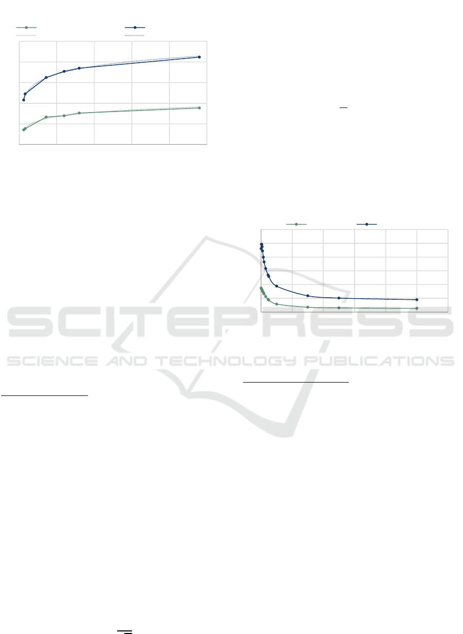
Figure 7: The average SNR as a function of the reference
powder region and the projection number.
Region 1 contained the silicate powder and
Region 2 contained the iron powder. Figure 4(left)
shows a cross-section of the powders with the
corresponding mask overlain on top of the data. To
determine the height of powders in two cylinders, we
assumed that the derivative of the average intensity of
each region per frame in the SIRT-2400pro dataset is
close to zero since the powders are homogeneous
along z-axis (corresponding to the cylinder height
dimension). The choice of a threshold for the derivate
to be close to zero was visually verified (SNR
threshold=0.000389) and resulted in defining the
powder z-slices to be in the [447, 514] range. Finally,
we calculated the signal-to-noise ratio (SNR) using
the definition in Equation (4).
SIRT-Xpro Dataset: The SNR method described
above was applied to the polychromatic datasets
reconstructed with the SIRT algorithm. The
differences in SNR values for Region 1 and Region 2
shown in Figure 4 (left) are due to the difference in
the average attenuation intensity of the regions, a
function of the properties of the reference powders,
and will vary depending on the homogenous material
being analyzed. Ranking both datasets from worst to
best quality we get: SIRT-60pro, SIRT-80pro,
SIRT-360pro, SIRT-600pro, SIRT-800pro, and
SIRT-2400pro. This ranking from lowest to highest
projection number was expected due to the Poisson
noise detailed below and helps validate the use of
SNR based evaluations for the other datasets.
As with most neutron imaging datasets, the noise
in the data is dominated by Poisson counting
statistics. Without any interaction with a sample, the
SNR is governed by the counting statistics according
to:
=
√
(6)
where is the number of incident neutrons
(Lewandowski et al., 2012). Thus, the increased
counting statistics with increasing number of
projections will increase the SNR value
exponentially. The application of the Beer-Lambert
Law in Equation below due to interaction with the
sample, transforms this into a logarithmic
relationship.
=
=
(7)
where is the measured intensity,
the incident
intensity, is the transmission, is the thickness, and
is the attenuation, a product of the neutron cross
section and the atom density (dependent on the
material). A predictive relationship between SNR and
the number of 2D projections can be derived from the
data shown in Figure 7.
Figure 8: The average SNR value on a single frame as a
function of the number of SIRT iterations with a seed.
SIRT+seed-Zpro Dataset: Applying the SIRT + seed
reconstruction method requires a trade-off between
accuracy, time, and image quality as in Fig. 6, Fig. 8
and Fig. 9 show the dependency of SNR and RMSE on
the SIRT iterations. Fig. 9 indicates that (a) the ground
truth 3D volume we compare against has lower image
quality with respect to RMSE error than the seed
volume, and (b) for the increased number of iterations,
the resulting 3D volume is deviating more from the
seed and converging closer to the 3D reconstruction
from the input projection images without the seed.
Thus, quality of the 3D reconstructed volume will vary
between the quality value of the seed and the quality
value of the input data as a function of the number of
iterations. However, utilizing this method would
dramatically decrease the time required to reconstruct
a dataset of similar quality. Using the SIRT + seed
method with 20 iterations would take about 7 minutes
for reconstruction and about 0.6 hours to collect and
yield image quality similar to the SIRT-360pro data set
that takes about 1.5 hours to reconstruct and 2.5 hours
to collect, a savings of over 3 hours per dataset, 2 hours
of which is expensive neutron acquisition time.
y = 1,4896ln(x) - 2,4873
R² = 0,9875
y = 2,7716ln(x) - 0,1681
R² = 0,9955
0
5
10
15
20
25
0 500 1000 1500 2000 2500
Average SNR
Number of 2D Projections
Average SNR(frames in [447,514])=f(Region,
Projection)
average SNR(R1) average SNR(R2)
Log. (average SNR(R1)) Log. (average SNR(R2))
0
5
10
15
20
25
30
0 200 400 600 800 1000 1200
Average SNR
SIRT Iterations
Average SNR (single 2D frame)
average SNR(R1) average SNR(R2)
IMPROVE 2022 - 2nd International Conference on Image Processing and Vision Engineering
72
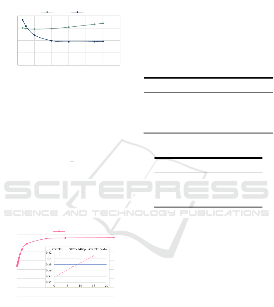
Fig
ure 9: The Root Mean Squared Error for the reference
powder regions as a function of the number of SIRT
iterations with a seed.
4.4 Blur based Comparisons
For the choice of optimal blur metric with maximum
variability (Assumption 1 from section 4.4), we
calculated the coefficient of variation (CV) for the
various blur metrics for the SIRT datasets according
to:
=
̅
(8)
where s is the sample standard deviation and ̅ is
the sample mean. The blur metrics with the highest
coefficient of variation for each dataset are selected
to provide the highest discrimination. Out of the six
datasets, the HELM blur metric was optimal for five
and hence it was selected as the optimal metric for
Assumption 1.
Figure 10: The CRETE blur metrics on a single frame
(frame index: 451) as a function of the number of iterations.
The insert shows a zoomed in version of the graph with
iterations from 1 to 15 and the CRETE value for the SIRT-
2400pro for the same frame (between 7 and 10 iterations).
For the choice of optimal blur metric aligned with
human perception (Assumption 2), we used the
CRETE method, which has been validated with a
human perception test (Crete et al., 2007b). As
expected, the dataset with largest number of
projections (SIRT-2400pro) had the lowest blur
metric (the best quality) and the blur metric generally
increased with decreasing projection number. The
exception being SIRT-60pro and SIRT-80pro which,
qualitatively, were similar throughout. Figure 10
illustrates the relationship between CRETE metric
and the SIRT iterations for a fixed z-frame applied to
the 3D reconstruction using monochromatic
SIRT+seed-Zpro dataset.
Table 1: Ranking of Datasets According to the Blur Metric.
Projections
Assumption 1
HELM
Assumption 2
CRETE
60 5 5
80 6 6
360 4 4
600 3 3
800 1 2
2400 2 1
Note: 1-6 from least blur to most blur
Table 2: CRETE Values.
Dataset
CRETE
Value
SIRT + seed: 20 iterations 0.43
SIRT-360pro 0.49
SIRT-600pro 0.48
SIRT-800pro 0.46
SIRT-2400pro 0.38
For both criteria for selecting optimal blur
metrics, the datasets were ranked according to the
average blur metric from 1 to 6, with 1 being the least
blurry. The results are shown in Table 1 . The
rankings for the HELM and blur metrics differed
slightly and were consistent for all but the SIRT-
2400pro and SIRT-800pro datasets. We expected the
SIRT-2400pro dataset to have the lowest blur metric
due to the higher number of projections, which was
the case for the CRETE method (see Table 2), but not
for the HELM metric. This lends credence to the
CRETE method of evaluating blur and will be the
main metric considered for the rest of this work.
Another deviation from the expected results is the
higher ranking of SIRT-60pro compared to SIRT-
80pro. This relationship is consistent in both the
HELM and the CRETE methods and could be due to
a smoothing out of features and boundaries in the
SIRT-60pro.
4.5 SNR and Blur for MS-D Net
Postprocessed Datasets
Lastly, we analyzed the machine learning post-
processing method for each trained network. We then
0
0,5
1
1,5
2
0 102030405060
RMS Error
SIRT Iterations
Root Mean Squared Error
Region 1 Region 2
0
0,1
0,2
0,3
0,4
0,5
0,6
0,7
0 200 400 600 800 1000
CRETE
…
SIRT Iterations
Blur Values for Single 2D Slice
CRETE
Assessment of Dose Reduction Strategies in Wavelength-selective Neutron Tomography
73
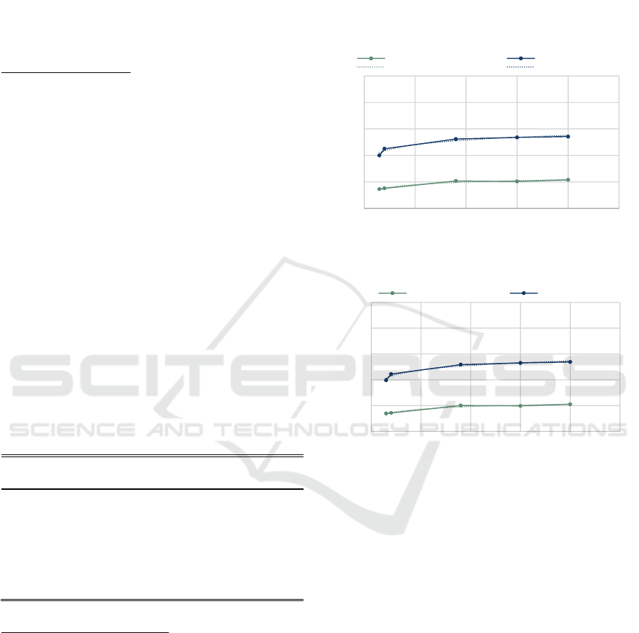
calculated the average SNR per calibration region for
each network as a function of the number of
projections using the same procedure as before (Fig.
11 A-C). Based on the SNR results, the network
performance can be divided into two groups that
show similar trends, the 60/80 MS-D Net data and the
360/600/800 MS-D Net data.
60/80 MS-D Net Data: The SNR results for these two
networks demonstrate that the best SNR ratio was
achieved when the MS-D Net was applied to the data
set it was trained on (Fig. 11 A). In the training data,
there were various degrees of artifacts due to the low
projection number. Each model was trained to
compensate for the degree of artifacts that were
present in the samples and did not perform as well
when the artifacts were not present or present but to a
lesser extent than the dataset it was trained on. When
compared to the original SIRT datasets, the maximum
SNR values were much higher than the original SNR
values (Table 3) and in the MS-D Net80 case, higher
that the SIRT-2400pro dataset. Thus, these networks
were able to improve the SNR of the original datasets.
The blur results using CRETE are a bit more
difficult to interpret because while the SNR
calculation is only applied to the homogenous
powders, the blur metric is calculated across the entire
volume, including the heterogenous rock samples.
Table 3: SNR Max Values, the SIRT datasets (last four
rows) only had one SNR value, whereas, for the MSD
networks (first three rows), the max SNR value for every
dataset was used.
Dataset/Network
SNR Max Value
Region 1
SNR Max Value
Region 2
MS-D Net360 5.38 13.56
MS-D Net600 5.99 13.25
MS-D Net800 5.24 13.45
SIRT-360pro 6.68 16.26
SIRT-600pro 7.00 17.76
SIRT-800pro 7.65 18.52
SIRT-2400pro 8.87 21.22
360/600/800 MS-D Net Data: The SNR results for the
360/600/800 MS-D Nets all show consistent results.
These networks did not perform well (low SNR
values) when applied to the SIRT- 60pro/80pro
datasets that contained reconstruction artifacts due to
low projection numbers. Since the networks were
trained with datasets that did not have many artifacts,
they were not trained to remove them. These artifacts
were thus still present in the data after the networks
were applied, leading to lower SNR values. The
networks performed best when they were applied to
the SIRT- 360pro/600pro/800pro datasets. When
compared to the original SIRT datasets, the maximum
SNR value for all three networks was below the SNR
value of the initial datasets (Table 3). Thus, these
networks were not able to make any improvements in
the SNR values.
Figure 11: The average SNR values for the MS-D Net
trained networks and 3D datasets reconstructed from 60,
360, and 800 projections.
5 DISCUSSION
This paper presented (1) an experimental design to
understand the trade-offs between acquisition time
and image quality of 3D tomographic reconstructions
from neutron imaging data, (2) evaluations of SNR,
RMSE, blur metrics, and intensity variance as the
measurements of image quality and their
relationships to acquisition parameters, and (3)
integration of the MS-D NN model-based denoising
to leverage previously acquired high quality dataset.
We have created several “ground truth” datasets and
included assumptions, models, and methods to
quantify several image quality metrics as listed in
Table 4.
Table 4 summarizes all relationships documented
in the experimental section. We could classify them
y = 0,6918ln(x) + 0,8131
R² = 0,9578
y = 1,2872ln(x) + 5,1938
R² = 0,9443
0
5
10
15
20
25
0 200 400 600 800 1000
Average SNR
Number of 2D Projections
B. MSDnet360
Average SNR(frames in
[447,514])=f(Region,Projection)
average SNR(R1) average SNR(R2)
Log. (average SNR(R1)) Log. (average SNR(R2))
y = 0,7112ln(x) + 0,5333
R² = 0,9623
y = 1,2819ln(x) + 5,0905
R² = 0,9513
0
5
10
15
20
25
0 200 400 600 800 1000
Average SNR
Number of 2D Projections
C. MSDnet800
Average SNR(frames in
[447,514])=f(Region,Projection)
average SNR(R1) average SNR(R2)
IMPROVE 2022 - 2nd International Conference on Image Processing and Vision Engineering
74

into linear, non-linear (logarithmic), and content
dependent. Due to a large spectrum of blur
definitions, one must consider ranking the blur
metrics, for example, based on the coefficient of
variation (CV). The ranking order becomes the first
step before a modelled relationship can be
established.
This work examined three separate methods of
improving 3D tomographic reconstructions at
neutron imaging beamlines: (1) one baseline
reconstruction method as a function of varying input
numbers of projections, (2) one method as a function
of incorporated seeds into an iterative 3D
reconstruction algorithm, and (3) one post-processing
method as a function of incorporated non-linear
mappings derived from existing datasets. The first
reconstruction algorithm (SIRT) established baseline
metrics for analyzing neutron tomograms, including
SNR and the CRETE blur metric. The second
reconstruction algorithm (SIRT + seed) used a high-
quality dataset to initialize the SIRT reconstruction.
The final approach, a post-processing method,
applied a machine learning algorithm (MS-D net) to
sharpen and de-noise the reconstruction images.
Using the metrics determined when analyzing the
SIRT datasets, we found that the SIRT + seed method
could utilize a high-quality dataset of similar
attenuation values and the same shape to reconstruct
unknown datasets with trade-offs between accuracy,
time, and image quality. As little as 20 iterations of
an 80-projection dataset was shown to improve image
quality comparable to a dataset with at least 360-
projections. Utilizing this method would dramatically
decrease the time required to reconstruct and collect
datasets, allowing more advanced neutron imaging
methods to be utilized.
The post-processing method using the MS-D Net
demonstrated the benefit of using this method for
low-projection datasets, especially if the algorithm is
trained on a dataset with the same number of
projections. These networks showed improvements in
SNR values and CRETE blur metrics that indicate
higher-quality data. However, as shown in the higher-
projection dataset, care must be taken when applying
machine learning models across multiple
configurations on the neutron imaging beamlines.
6 CONCLUSIONS
This paper presented (1) an experimental design to
understand the trade-offs between acquisition time
and image quality of 3D tomographic reconstructions
from neutron imaging data, (2) evaluations of SNR,
RMSE, blur metrics, and intensity variance as the
measurements of image quality and their
relationships to acquisition parameters, and (3)
integration of the MS-D NN model-based denoising
to leverage previously acquired high quality dataset.
We have created several “ground truth” datasets and
included assumptions, models, and methods to
quantify several image quality metrics as listed in
Table 4.
Table 4: Summary of explored relationships and rankings.
GT is ground truth, “A priori” refers to assumptions &
models, and methods, M denotes the number of 2D
projections, N is the number of SIRT iterations, RM is
reference segmentation mask, RV is reference 2400
projection-based 3D reconstruction, RP is reference
powders, and MS-D is mixed-scale dense neural network
trained model.
Relationship
Dependent
var.
Independent
var.
A priori
GT
Datasets
Linear Acq. time M
Linear:
Eq. (5)
Time to
reconstruct
volume
N
Linear:
Figure 5
Intensity
Variance
1/M Cylinders RP
Log:
Figure 7
SNR M
RP &
SIRT-Xpro
method
RM
Linear:
Figure 8
SNR N
RP &
SIRT+seed
-Zpro
method
RM
Ranking:
Figure 9
Min RMSE
over
powders
N & intensity
RP &
SIRT+seed
-Zpro
method
RM &
RV
Log:
Figure 10
CRETE
Blur
N
SIRT+seed
-Zpro
method &
MS-D
RV
Log:
Figure 11
SNR M, RP type
SIRT+seed
-Zpro
method &
MS-D &
RP
RM &
RV
The paper aims at identifying trade-offs between
3D reconstruction quality and acquisition time by
discovering relationships among variables measuring
several aspects of imaging, such as acquisition speed,
imaging focus, object discrimination from
background, 3D reconstruction method, and noise
modelling. Once the models for relationships are
established and parametrized, a user can choose a
compromise between acquisition time and accuracy
of the final measurement depending on 3D
reconstruction quality. Thus, the analysis completed
Assessment of Dose Reduction Strategies in Wavelength-selective Neutron Tomography
75

here may help users of neutron beam facilities to plan
and carry out experiments at the neutron imaging
beamline. The work is also intended to be an initial
look at how the 3D reconstruction techniques could
be used at neutron imaging facilities to improve 3D
reconstructions with additional seeding and
supervised model-based denoising.
DISCLAIMER
Certain commercial equipment, instruments, or
materials (or suppliers, or software, ...) are identified
in this paper to foster understanding. Such
identification does not imply recommendation or
endorsement by the National Institute of Standards
and Technology, nor does it imply that the materials
or equipment identified are necessarily the best
available for the purpose.
REFERENCES
Bingham, P., Polsky, Y., & Anovitz, L. (2013). Neutron
imaging for geothermal energy systems. In P. R.
Bingham & E. Y. Lam (Eds.), Image Processing:
Machine Vision Applications VI (Vol. 8661, Issue 6, p.
86610K). SPIE. https://doi.org/10.1117/12.2004617
Brooks, A. J., Knapp, G. L., Yuan, J., Lowery, C. G., Pan,
M., Cadigan, B. E., Guo, S., Hussey, D. S., & Butler, L.
G. (2017). Neutron imaging of laser melted SS316 test
objects with spatially resolved small angle neutron
scattering. Journal of Imaging, 3(4), 1–11.
https://doi.org/10.3390/jimaging3040058
Chen, Y., Zhang, Y., Zhang, K., Deng, Y., Wang, S.,
Zhang, F., & Sun, F. (2016). FIRT: Filtered iterative
reconstruction technique with information restoration.
Journal of Structural Biology, 195(1), 49–61.
https://doi.org/10.1016/j.jsb.2016.04.015
Crete, F., Dolmiere, T., Ladret, P., & Nicolas, M. (2007a).
The blur effect: perception and estimation with a new
no-reference perceptual blur metric. In B. E. Rogowitz,
T. N. Pappas, & S. J. Daly (Eds.), Human Vision and
Electronic Imaging XII (Vol. 6492, p. 64920I). SPIE.
https://doi.org/10.1117/12.702790
Crete, F., Dolmiere, T., Ladret, P., & Nicolas, M. (2007b).
The blur effect: perception and estimation with a new
no-reference perceptual blur metric. In B. E. Rogowitz,
T. N. Pappas, & S. J. Daly (Eds.), Human Vision and
Electronic Imaging XII (Vol. 6492, p. 64920I). SPIE.
https://doi.org/10.1117/12.702790
Gates, C. H., Perfect, E., Lokitz, B. S., Brabazon, J. W.,
McKay, L. D., & Tyner, J. S. (2018). Transient analysis
of advancing contact angle measurements on polished
rock surfaces. Advances in Water Resources, 119, 142–
149. https://doi.org/10.1016/j.advwatres.2018.03.017
Hilger, A., Manke, I., Kardjilov, N., Osenberg, M.,
Markötter, H., & Banhart, J. (2018). Tensorial neutron
tomography of three-dimensional magnetic vector
fields in bulk materials. Nature Communications, 9(1),
1–7. https://doi.org/10.1038/s41467-018-06593-4
Hussey, D. S., Brocker, C., Cook, J. C., Jacobson, D. L.,
Gentile, T. R., Chen, W. C., Baltic, E., Baxter, D. V.,
Doskow, J., & Arif, M. (2015). A New Cold Neutron
Imaging Instrument at NIST. Physics Procedia, 69.
https://doi.org/10.1016/j.phpro.2015.07.006
Jau, Y. Y., Hussey, D. S., Gentile, T. R., & Chen, W.
(2020). Electric field imaging using polarized neutrons.
ArXiv, 3.
Kak, A. C., Slaney, M., & Wang, G. (2002). Principles of
Computerized Tomographic Imaging. Medical Physics,
29(1), 107–107. https://doi.org/10.1118/1.1455742
Kak, A.C., S. M. (n.d.). Principles of Tombgraphic
Imaging. Book.
Lewandowski, R., Cao, L., & Turkoglu, D. (2012). Noise
evaluation of a digital neutron imaging device. Nuclear
Instruments and Methods in Physics Research, Section
A: Accelerators, Spectrometers, Detectors and
Associated Equipment, 674, 46–50.
https://doi.org/10.1016/j.nima.2012.01.025
NIST Disclaimer Statement/NIST. (n.d.).
https://www.nist.gov/disclaimer
Palenstijn, W. J., Batenburg, K. J., & Sijbers, J. (2011a).
Performance improvements for iterative electron
tomography reconstruction using graphics processing
units (GPUs). Journal of Structural Biology, 176(2),
250–253.
Palenstijn, W. J., Batenburg, K. J., & Sijbers, J. (2011b).
Performance improvements for iterative electron
tomography reconstruction using graphics processing
units (GPUs). Journal of Structural Biology, 176(2),
250–253. https://doi.org/10.1016/j.jsb.2011.07.017
Pelt, D. M., & Sethian, J. A. (2017). A mixed-scale dense
convolutional neural network for image analysis.
Proceedings of the National Academy of Sciences of the
United States of America, 115(2), 254–259.
https://doi.org/10.1073/pnas.1715832114
Petruccelli, J. C., Tian, L., & Barbastathis, G. (n.d.).
imaging. 2, 2–4.
Rauch, H., & Werner, S. A. (2015). Neutron Interferometry
2nd Edn. In Neutron Interferometry 2nd Edn. Oxford
University Press. https://doi.org/10.1093/acprof:oso/
9780198712510.001.0001
Schofield, R., King, L., Tayal, U., Castellano, I., Stirrup, J.,
Pontana, F., Earls, J., & Nicol, E. (2020). Image
reconstruction: Part 1-understanding filtered back
projection, noise and image acquisition.
https://doi.org/10.1016/j.jcct.2019.04.008
Strobl, M. (2014). General solution for quantitative dark-
field contrast imaging with grating interferometers.
Scientific Reports, 4(1), art. no. 7243.
https://doi.org/10.1038/srep07243
Tayal, U., King, L., Schofield, R., Castellano, I., Stirrup, J.,
Pontana, F., Earls, J., & Nicol, E. (2019). Image
reconstruction in cardiovascular CT: Part 2-Iterative
reconstruction; potential and pitfalls.
https://doi.org/10.1016/j.jcct.2019.04.009
IMPROVE 2022 - 2nd International Conference on Image Processing and Vision Engineering
76

Van Aarle, W., Palenstijn, W. J., Cant, J., Janssens, E.,
Bleichrodt, F., Dabravolski, A., De Beenhouwer, J.,
Batenburg, K. J., & Sijbers, J. (2016a). Fast and flexible
X-ray tomography using the ASTRA toolbox. Optics
Express, 24(22), 25129–25147.
Van Aarle, W., Palenstijn, W. J., Cant, J., Janssens, E.,
Bleichrodt, F., Dabravolski, A., De Beenhouwer, J.,
Batenburg, K. J., & Sijbers, J. (2016b). Fast and flexible
X-ray tomography using the ASTRA toolbox. Optics
Express, 24(22), 25129–25147.
van Aarle, W., Palenstijn, W. J., Cant, J., Janssens, E.,
Bleichrodt, F., Dabravolski, A., De Beenhouwer, J.,
Joost Batenburg, K., & Sijbers, J. (2016). Fast and
flexible X-ray tomography using the ASTRA toolbox.
Optics Express, 24(22), 25129.
https://doi.org/10.1364/oe.24.025129
Van Aarle, W., Palenstijn, W. J., De Beenhouwer, J.,
Altantzis, T., Bals, S., Batenburg, K. J., & Sijbers, J.
(2015a). The ASTRA Toolbox: A platform for
advanced algorithm development in electron
tomography. Ultramicroscopy, 157, 35–47.
Van Aarle, W., Palenstijn, W. J., De Beenhouwer, J.,
Altantzis, T., Bals, S., Batenburg, K. J., & Sijbers, J.
(2015b). The ASTRA Toolbox: A platform for
advanced algorithm development in electron
tomography. Ultramicroscopy, 157, 35–47.
Vitucci, G., Minniti, T., Di Martino, D., Musa, M., Gori, L.,
Micieli, D., Kockelmann, W., Watanabe, K., Tremsin,
A. S., & Gorini, G. (2018). Energy-resolved neutron
tomography of an unconventional cultured pearl at a
pulsed spallation source using a microchannel plate
camera. Microchemical Journal, 137, 473–479.
https://doi.org/10.1016/j.microc.2017.12.002
Vo, N. T., Atwood, R. C., & Drakopoulos, M. (2018).
Superior techniques for eliminating ring artifacts in X-
ray micro-tomography. Optics Express, 26(22), 28396.
https://doi.org/10.1364/OE.26.028396
Woracek, R., Penumadu, D., Kardjilov, N., Hilger, A.,
Boin, M., Banhart, J., & Manke, I. (2014). 3D Mapping
of Crystallographic Phase Distribution using Energy-
Selective Neutron Tomography. Adv. Mater.
(Weinheim, Ger.), 26(24), 4069–4073.
Gavin D. Peckham and Ian J. McNaught, Applications of
Maxwell-Boltzmann distribution diagrams, Journal of
Chemical Education 1992 69 (7), 554, DOI:
10.1021/ed069p554
Oxford Instruments, Andor’s fast and sensitive sCMOS
cameras, URL: https://andor.oxinst.com/products/fast-
and-sensitive-scmos-cameras
S. Pertuz, D. Puig, and M. A. Garcia, “Analysis of focus
measure operators for shape-from-focus,” Pattern
Recognit., vol. 46, no. 5, pp. 1415–1432, May 2013,
doi: 10.1016/j.patcog.2012.11.011.
Assessment of Dose Reduction Strategies in Wavelength-selective Neutron Tomography
77
