
Metrics of Parallel Complexity of Operational Business Processes
Andrea Chiorrini, Claudia Diamantini, Alex Mircoli and Domenico Potena
Department of Information Engineering, Polytechnic University of Marche, Ancona, Italy
Keywords:
Business Modelling, Business Process Management, Metrics and Evaluation of Processes, Degree of
Parallelism, Instance Graphs.
Abstract:
This paper addresses the problem of quantifying the parallelism in a business process. Having a synthetic
metric to quantify the parallelism of a process may provide an assessment of the complexity of the process and
guide certain design choice. In the present paper we discuss the advantages and disadvantages of two metrics
presented in the literature, as well of two novel metrics that leverage on the notion of Instance Graph. Analysis
is performed by means of use cases that are representative of operational business processes. The proposed
metrics show to provide a sensible way to evaluate the overall parallel complexity of a process model.
1 INTRODUCTION
A business process is a flow of related activities ex-
ecuted by people and/or machines to achieve a spe-
cific goal for a client. Activities can be executed
sequentially, or in parallel, and cycles may exist as
well. Business process modelling is a fundamental
task in business management since it allows to de-
sign, analyse and improve process efficiency. Sev-
eral metrics have been devised to measure relevant
aspects of business processes (Radu Mateescu, 2014;
Mao, 2010). Among them, one of particular interest
is how much parallel a process is. It is acknowledged
that increasing the number of activities performed in
parallel is a way to improve the performance of a
business process (Davenport, 1993), although this im-
provement comes at the cost of a more complex pro-
cess design, development, and maintenance. Hav-
ing a synthetic metric to quantify the parallelism of
a process may thus provide an assessment of the pro-
cess and guide certain design choices. In the litera-
ture, a widely adopted metric is the Degree of Par-
allelism (DoP), defined as the maximum number of
parallel activities that can be executed in that process
(Radu Mateescu, 2014; Sun and Su., 2011). In par-
ticular, (Sun and Su., 2011) proposes different algo-
rithms to compute the DoP for three classes of BPMN
processes. In (Radu Mateescu, 2014) it is observed
that the DoP, theoretically, can be computed by deter-
mining the bound of a Petri net, which is the maxi-
mum number of tokens in a marking of the net. The
computation of such bound requires the construction
of the reachability graph, whose derivation is known
to be an NP-complete problem or ever harder for some
classes of Petri nets (Esparza, 1998; Mayr., 1984).
A more efficient general procedure is then proposed
for a wide class of BPMN processes, which exploits
the notion of Labeled Transition System and model
checking. An extension (Dur
´
an et al., 2018) con-
siders timed business processes modeled in BPMN,
where execution times are associated to BPMN con-
structs such as activities and flows. The DoP metric
is concerned with the “worst” case scenario. Other
metrics aimed at assessing the overall complexity of
a business process are discussed in (Mao, 2010). In
particular, it is argued that complexity of the paral-
lelism of a process can be measured by the Average
Degree of Transitions (ADT) which is the average
number of incoming and outgoing arcs of transitions
in a Petri net. In the present paper we discuss the ad-
vantages and disadvantages of these two metrics and
we propose two novel metrics to measure the over-
all parallel complexity of a process by leveraging on
the notion of Instance Graph (IG). We show that these
two novel metrics manage to capture the advantages
of both DoP and ADT and we discuss their pros and
cons by means of use cases that are representative of
operational business processes modelled by a class of
Petri Nets called Workflow Nets (Aalst, 1997).
The rest of the paper is organised as follows: in
Section 2 we briefly recall the notions of Petri Nets
and IGs. Section 3 describes the set of processes con-
sidered as use cases for assessment purpose. Then,
Section 4 is devoted to the definition and comparison
Chiorrini, A., Diamantini, C., Mircoli, A. and Potena, D.
Metrics of Parallel Complexity of Operational Business Processes.
DOI: 10.5220/0011084200003179
In Proceedings of the 24th International Conference on Enterprise Information Systems (ICEIS 2022) - Volume 2, pages 561-566
ISBN: 978-989-758-569-2; ISSN: 2184-4992
Copyright
c
2022 by SCITEPRESS – Science and Technology Publications, Lda. All rights reserved
561

Figure 1: An example of: Petri net (a), Instance Graph (b),
variants (c).
of DoP, ADT and the two novel metrics. Finally, Sec-
tion 5 provides some final remarks and sketches future
work.
2 PRELIMINARIES
A business process is a flow of related activities exe-
cuted by people and/or machines to achieve a specific
output for a client. Activities can be executed sequen-
tially, or in parallel and loops can exist. In the present
paper we will focus on loop-free processes. A process
model is a general description of the flow of activities.
Several notations exist to describe a process model,
like Petri nets (van der Aalst and van Hee, 1996), or
BPMN (van der Aalst, 2018). In the following we
will discuss the properties of the different metrics on
a set of paradigmatic processes described in Petri nets
notation.
Figure 1(a) shows a simple Petri net. Squares rep-
resent transitions, that is well-defined activities that
have to be performed within the process. Circles rep-
resent places, that can be informally interpreted as re-
sources or pre-conditions enabling transitions. The
availability of a set of resources is denoted by a mark-
ing (the black dot in the figure). Arcs connecting
places to transitions describe the set of resources that
must be available in order to perform the activity,
while arcs connecting transitions to places describe
the set of resources enabled by the effect of activity
execution. Hence, from the marking shown, only one
between the activity t1 and t2 can be performed at
each process execution (we say that t1 and t2 are al-
ternative choices). If t1 is performed then t3 and t4
are both enabled, this represents an interleaving be-
haviour that allow to perform in parallel the two ac-
tivities. Finally, their execution enables t5 which ends
the process. Note that we focus on operational busi-
ness processes, that are represented by a sub-class of
Petri nets called Workflow nets (WF-net). A WF-net
has one start place, one end place, and all transitions
and all places are on a path from start to end.
A specific execution of the process generates a so-
called process instance, which is the partially ordered
set of activities that are performed to achieve the com-
pletion of a single execution of a process. A process
instance can be modelled by an IG. In an IG each node
represents an activity, and an edge between activity A
and activity B denotes the existence of a causal rela-
tion between A and B, namely the fact that B cannot
be executed until A is terminated; in other words, the
execution of B depends on the execution of A. For a
more formal definition of IGs and causal relations see
(van Dongen and van der Aalst, 2004). The IG cor-
responding to the upper part of the Petri net in Figure
1(a) (marked by a square) is shown in 1(b), while the
IG for the lower part is simply a node labelled t2. In
an IG, all control-flow structures are represented ex-
cept for choices. This is obvious, since in each single
execution choices have already been made. Activities
that can be done in parallel within one instance can be
executed in any order. As a consequence, an IG is rep-
resentative of one or more variants that differ exactly
in the interleaving of parallel activities. The variants
for the IG in Figure 1(b) are reported in Figure 1(c).
The relation between an IG and its underlying variants
is the basic property underpinning the development of
the metrics proposed in this work.
3 USE CASES DESCRIPTION
In this section we introduce 7 use cases, in the form
of Petri nets. Although simple, these processes have
been designed to capture some paradigmatic situa-
tions allowing to enlighten the properties of the dif-
ferent metrics, and can be easily scaled. Table 1 de-
scribes the characteristics of the processes. The pro-
cesses are shown in Figures 2-8. In particular, we de-
signed use case 1 (Fig. 2), as a simple starting base
case so to compare the added structural complexity of
the other models with it. Use case 2, (Fig. 3) only
adds to use case 1 a sequence of transitions after the
parallelism. Hence, for this model, it is desirable that
a metric lowers its score. Concerning use case 3 (Fig.
4), we designed it to highlight the opposite behaviour:
it is basically a sequence of two use case 1, so it would
be reasonable to see an increase in the metric score.
Use case 4 (Fig. 5), has been designed so to compare
it with both use cases 2 and 3. We expect to see an
increased score w.r.t. the former, while it is more dif-
ficult to compare the quantity of parallelism with the
latter. Indeed, use case 4 has a greater number of ac-
ICEIS 2022 - 24th International Conference on Enterprise Information Systems
562

Figure 2: Use case 1.
tivities that can be performed simultaneously, while
use case 3 has a greater number of parallelisms. Sim-
ilarly, we designed use case 5 (Fig. 6) as a problem-
atic example to compare with use cases 1 and 2, since
there are a greater number of activities in the parallel
branch. Use case 6 (Fig. 7) is introduced to show the
effect of synchronisation on the parallel complexity
of the process with respect to use case 5. Lastly, we
consider use case 7 (Fig. 8) to show the effects of an
or split on the various metrics.
4 METRICS FOR PROCESS
PARALLELISM EVALUATION
4.1 Metrics based on Model Perspective
In this subsection we introduce two popular metrics,
whose values are calculated directly from the struc-
ture of the process.
4.1.1 Average Degree of Transition
The Average Degree of Transition (ADT) has been
introduced in the context of Petri net-based business
process as a mean to measure control flow parallel
complexity (Mao, 2010). It is defined as:
ADT =
∑
T
i
deg(t
i
)
|T |
(1)
where T is the set of all transitions in the Petri net, and
deg : T → N is the function that associates to a transi-
tion the number of its incoming and outgoing arcs. It
is relevant to notice that such metric assumes values
in [2;+∞), a value of 2 represents a purely sequen-
tial process whereas bigger values indicate the pres-
ence of more parallelism. As examples, considering
use case 1 we can compute the ADT as 10/4 = 2.5
whereas for the use case 2 it is 16/7 = 2.29.
4.1.2 Degree of Parallelism
The most commonly used metric to quantify the par-
allelism of a process is the maximum number of ac-
tivities that can be executed in parallel, called Degree
of Parallelism (DoP). It is computed by evaluating the
number of activities enabled by a marking of the Petri
net. For examples, for the use case 1 the value of DoP
is 2 due to the marking
h
p1, p3
i
which enables both
transitions t2 and t4; for the process in Figure 5 the
DoP is 3 since the marking
h
p1, p6, p8
i
enables the
maximum number of transitions, namely t2,t7 and t8.
Techniques to calculate the DoP have been proposed
in (Radu Mateescu, 2014; Sun and Su., 2011).
4.1.3 Comparison between DoP and ADT
First of all we notice that as the DoP calculate a max-
imum parallelism, it is hence suited to assess peak be-
haviours, whereas ADT shows a more comprehensive
average complexity of the process. In order to high-
light this fact, let us consider use cases 2 and 3. The
value of the DoP metric is 2 for both processes, but the
latter clearly shows a more complex behaviour due to
the presence of a second parallelism. This is captured
by ADT whose value is increased from 2.29 to 2.5.
Clearly DoP is able to capture the difference between
processes in Figures 3 and 5 passing from 2 to 3. ADT
also detect the increased complexity, although with a
slightly minor relative increment passing from 2.29 to
2.5. We remark that the ADT metric returns the same
value for use cases 3 and 4, demonstrating that ADT
is unable to capture the increased complexity inherent
to a parallelism with a higher number of parallel activ-
ities. The values of DoP and ADT metrics for all the
use cases are shown in the last two columns of Table
2. The limits discussed for the two metrics motivated
us to focus on a different aspect of a process model to
define a metric. Specifically, in the following subsec-
tion we describe two metrics which take into account
the number of variants represented by an IG.
4.2 Metrics based on Instance Graphs
We can say that each IG represents a specific set of
parallel branches that exist in the process and that the
parallel complexity of such set is as high as the num-
ber of variants represented by the IG. On this basis
we introduce a metric called Parallel Complexity, and
a scaled variant, designed to overcome the limits of
both ADT and DoP being more sensitive to both over-
all and maximum parallelism.
4.2.1 Parallel Complexity (PC)
This metric is defined as:
PC =
|V |
|IG|
− 1 (2)
where |V | is the number of distinct variants allowed
by the process model and |IG| is the number of dis-
tinct IGs that represents those variants. The minus 1
Metrics of Parallel Complexity of Operational Business Processes
563

Table 1: Use case descriptions.
Process Description
Use case 1 a process with 2 parallel activities (simple parallelism)
Use case 2 a process with 2 parallel activities followed by a sequence
Use case 3 a process with a sequence of 2 simple parallelisms
Use case 4 a process with 3 parallel activities followed by a sequence
Use case 5 a process with two parallel sequences followed by a further sequence
Use case 6 use case 5 with a synchronisation between activities t7 and t3
Use case 7 a process with an alternative choice between use case 1 and use case 5
Figure 3: Use case 2.
is a scaling parameter used to reduce to 0 the Paral-
lel Complexity in case of strictly sequential processes.
Given a process model, the set of IGs can be easily ob-
tained by a two-step procedure. First, the variants of a
process are generated (play-out). Then, using causal
relations of the model, an IG is generated for each
variant. Computing such metric for the provided use
cases, we can see that the metric shows an hybrid be-
haviour with respect to DoP and ADT, i.e., it is sen-
sitive to both overall parallelism and maximum paral-
lelism. On the one hand, as regards the use cases 2
and 3 we can notice that PC scores respectively 1 and
3 managing to reflect the increased overall parallelism
as ADT does, but DoP does not. On the other hand,
for use cases 3 and 4, PC takes the values 3 and 5
respectively, highlighting the difference between the
two examples as DoP does but ADT does not. Agree-
ing behaviours are displayed considering use cases 2
and 4 as both ADT and DoP detect the increment.
However, it should be noted that PC scores a bigger
relative increase. Indeed, the percentage increment of
ADT, DoP and PC are 9.2%, 50% and 400%, respec-
tively. This is due to the fact that adding a branch
to a parallelism does not increase linearly its com-
plexity as the possible actual executions of such par-
allelism grow combinatorially. A relevant advantage
of the PC metric is shown comparing use case 6 with
use case 5. The former adds to the latter a synchro-
nisation place p9 which locks the execution of t3 to
t7, therefore reducing the existing parallelism. In this
situation, ADT, instead of a reduction, even scores an
increment due to the arcs used to connect p9. DoP ig-
nore the change altogether. On the contrary we note
that PC correctly reflects the change passing from 5
of Figure 6 to 4 of Figure 7. A similar situation is
displayed by use cases 3 and 5, where ADT lowers
its value instead of increasing it. Use case in Figure
8 shows that PC also works well if choices exist in
the process model, giving rise to more than one IG.
Since this use case is composed by a choice between
1 and 5, PC correctly returns a score of 3 which is the
average of its values for these two use cases. A simi-
lar behaviour is displayed by ADT which scores 2.33
which is in-between the composing use cases ADT
values. The main limit of PC is that it doesn’t scale
well with respect to process length. To explain the
point, let us consider use cases 1 and 2. The former
shows a higher overall parallelism, since a larger por-
tion of process 2 is strictly sequential. Instead, PC
values for both processes is 1, whereas this difference
is captured by ADT. This motivates the introduction
of a scaled variant of the PC.
4.2.2 Scaled Parallel Complexity (SPC)
In order to overcome the described limit of the pro-
posed metric, we devised a scaling mechanism that
takes into account the number of activities.
SPC =
PC
(|T | − |S|)
(3)
where |T | is the total number of transitions in the
model and |S| is the number of transitions that have
more than one outgoing or incoming arcs. They in
fact represent the point where a parallel branch starts
(AND split) and where a parallel branch synchronises
(AND merge) respectively. From equation (2) we can
also write SPC as:
SPC =
|V | − |IG|
|IG|(|T | − |S|)
(4)
ICEIS 2022 - 24th International Conference on Enterprise Information Systems
564

Figure 4: Use case 3.
Figure 5: Use case 4.
Table 2: Metrics for all use cases.
Case |IG| |V | |T | |S| PC SPC ADT DoP
1 1 2 4 2 1 0.5 2.5 2
2 1 2 7 2 1 0.2 2.29 2
3 1 4 8 4 3 0.75 2.5 2
4 1 6 8 2 5 0.83 2.5 3
5 1 6 8 2 5 0.83 2.25 2
6 1 5 8 3 4 0.8 2.5 2
7 2 8 12 4 3 0.375 2.33 2
We can see from Table 2 that this new metric main-
tains all the good behaviours that PC has. It also dis-
plays the desired behaviour that PC does not have:
when considering use cases 1 and 2, we can note that
SPC decreases as required thanks to the scaling factor
that takes into account the presence of the sequence
in use case 2. We also notice that this scaling leads to
smaller relative increment with respect to PC. In con-
trast to PC, when considering use case 7 we see that
SPC fails to produce a coherent value. Indeed, use
case 7 is a process with an alternative choice between
use case 1 and use case 5. Nevertheless, SPC score
drops to 0.375 which is not in the range of scores for
use cases 1 and 5. This is due to how the scaling is
implemented. Currently the mechanism considers all
transitions in the process model even though the num-
ber of transitions in the derived IG could be far less.
This is because an IG only displays the activities from
one of the optional branches of the process. This over-
reduces the score by over-estimating the denominator
of SPC formula.
5 DISCUSSION AND
CONCLUSIONS
This paper addresses the problem of evaluating the
level of parallelism in a business process. We discuss
the limits of the two best known metrics in the liter-
ature and we introduce the Process Complexity met-
ric, and its scaled variant, based on the notion of In-
stance Graph. The idea underlying the proposed met-
ric is that the parallel complexity of a process linearly
depends on the number of distinct variants allowed
by each IG, representing the possible executions of
the process. This metric provides a sensible way to
evaluate the overall complexity of the process model
due to the number and structural relations among par-
allel activities. None of the metrics, on the other
hand, is fully satisfactory showing some incoherent
behaviours with respect to the number of activities
or the presence of alternative branches. One possi-
ble conclusion is that more than one metric should be
taken into account when evaluating the parallelism of
a process. The results are not conclusive as they have
been obtained on a set of synthetic use cases. Future
works will be devoted to confirm the result both the-
oretically and empirically on a larger set of process
models. Another research direction is toward the in-
troduction of different scaling mechanisms that takes
the length of a sequence of activities into due consid-
eration.
Metrics of Parallel Complexity of Operational Business Processes
565
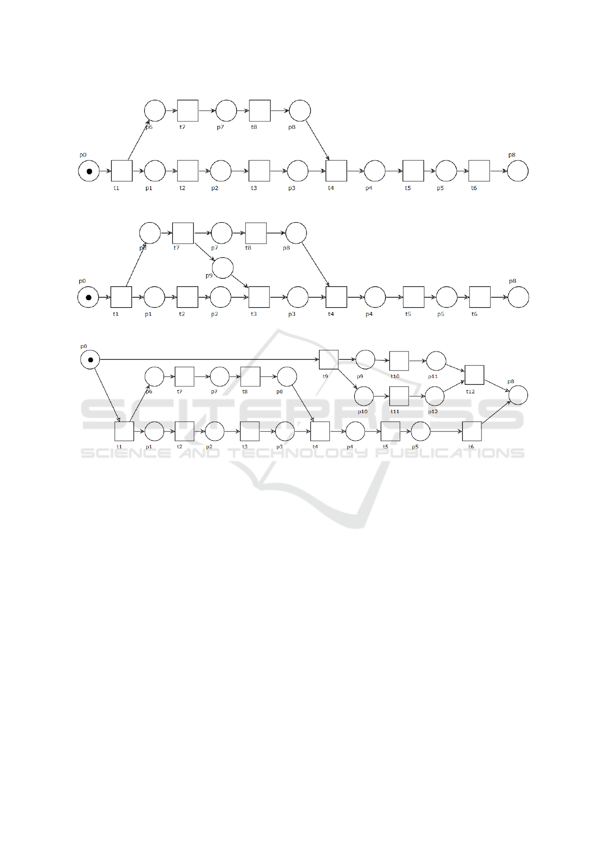
Figure 6: Use case 5.
Figure 7: Use case 6.
Figure 8: Use case 7.
REFERENCES
Aalst, W. (1997). Verification of workflow nets. In ICATPN,
pages 407–426.
Davenport, T. H. (1993). Process innovation: reengineering
work through information technology. Harvard Busi-
ness Press.
Dur
´
an, F., Rocha, C., and Sala
¨
un, G. (2018). Comput-
ing the parallelism degree of timed bpmn processes.
In Software Technologies: Applications and Founda-
tions, pages 320–335, Cham. Springer International
Publishing.
Esparza, J. (1998). Reachability in live and safe free-choice
Petri Nets is NP-complete. Theoretical Computer Sci-
ence.
Mao, C. (2010). Control flow complexity metrics for Petri
Net-based web service composition. Journal of Soft-
ware, 5:1292–1299.
Mayr., E. (1984). An algorithm for the general Petri Net
reachability problem. SIAM Journal on Computing.
Radu Mateescu, Gwen Sala
¨
un, L. Y. (2014). Quantify-
ing the parallelism in BPMN processes using model
checking. In The 17th International ACM Sigsoft Sym-
posium on Component-Based Software Engineering
(CBSE 2014).
Sun, Y. and Su., J. (2011). Computing degree of parallelism
for BPMN processes. In Springer, editor, Proceedings
of ICSOC’11, page 1–15.
van der Aalst, W. (2018). Business process modeling nota-
tion. In Liu, L. and
¨
Ozsu, M. T., editors, Encyclopedia
of Database Systems, pages 382–383. Springer New
York, New York, NY.
van der Aalst, W. and van Hee, K. (1996). Business process
redesign: A petri-net-based approach. Computers in
Industry, 29(1):15–26.
van Dongen, B. F. and van der Aalst, W. M. P.
(2004). Multi-phase process mining: Building in-
stance graphs. In Conceptual Modeling – ER 2004,
pages 362–376, Berlin, Heidelberg. Springer Berlin
Heidelberg.
ICEIS 2022 - 24th International Conference on Enterprise Information Systems
566
