
Deterministic Operating Strategy for Multi-objective NMPC for Safe
Autonomous Driving in Urban Traffic
Mostafa Emam and Matthias Gerdts
Department of Aerospace Engineering, Institute of Mathematics and Applied Computing,
Universitat der Bundeswehr Munchen, 85579, Neubiberg, Germany
Keywords:
Autonomous Driving, Multi-objective NMPC, Path Tracking, Finite-State Machine.
Abstract:
In this paper, we introduce a deterministic operating methodology based on finite-state automata to employ
multi-objective Nonlinear Model Predictive Control (NMPC) in autonomous driving applications. We begin
with discussing the system’s dynamical behavior and the proposed constraints to guarantee safe driving. Then,
we examine a typical urban scenario and dissect it into a set of interacting sequences, so that we develop and
fine-tune separate MPC-based controllers for each of these sequences. Finally, we introduce a Finite-State
Machine (FSM) that analyzes the current driving situation and accordingly selects the appropriate controller
to compute the optimal control action. This approach is numerically simulated and tested with the software
OCPID-DAE1 and results show its success in accordance with multi-objective NMPC.
NOMENCLATURE
Abbreviations
ACC Adaptive Cruise Control
FSM Finite-State Machine
LKA Lane Keeping Assistant
MIP Mixed-Integer Programming
MPC Model Predictive Control
NMPC Nonlinear Model Predictive Control
FSM States
ND End (Final state)
NP Enter Parking
PF Path Following
PU Pulling Up
SS Standstill
XP Exit Parking
1 INTRODUCTION
Over the past years, autonomous driving has become
an increasingly popular topic both in academia and
industry due to its many advantages, such as improving
road safety, optimizing fuel/energy consumption, and
enhancing the overall traveling experience (Lu et al.,
2004). This interdisciplinary topic requires intensive
research in diverse fields like environment perception,
sensor data fusion, and control theory, which is why
the quest for a system with full automation capabilities
is still incomplete to this day. Nonetheless, multiple
specialized systems have been successfully developed
to fulfill specific objectives, such as Adaptive Cruise
Control (ACC) and Lane Keeping Assistant (LKA),
and are currently being used in commercial vehicles
with great success (Yurtsever et al., 2020). So, in
this work we focus on the design of a path tracking
control algorithm with collision-avoidance capabilities,
in which we use NMPC as the control strategy due to
its flexibility and wide applicability (Gerdts, 2018).
(Luo et al., 2010) proposes an ACC system based
on multi-objective MPC that combines safety, comfort,
and economic objectives, yet it formulates the vehicle
longitudinal dynamics linearly, which greatly restricts
its applicability. (Chen et al., 2021) continues with the
same model and introduces a Finite-State Machine
(FSM) to accommodate for more complex driving
scenarios, which yields improved results but does not
fully represent the ego-vehicle’s lateral dynamics, thus
producing sub-optimal results when following curved
trajectories. Alternatively, (Zhang et al., 2017) uses a
vehicle model with longitudinal and lateral dynamics
and proposes a multi-objective FSM-based control
scheme that encourages lane changing when driving
behind a slower vehicle. However, the model implies
independent vehicle dynamics, which may generate
152
Emam, M. and Gerdts, M.
Deterministic Operating Strategy for Multi-objective NMPC for Safe Autonomous Driving in Urban Traffic.
DOI: 10.5220/0011115400003191
In Proceedings of the 8th International Conference on Vehicle Technology and Intelligent Transport Systems (VEHITS 2022), pages 152-161
ISBN: 978-989-758-573-9; ISSN: 2184-495X
Copyright
c
2022 by SCITEPRESS – Science and Technology Publications, Lda. All rights reserved

infeasible trajectories in real applications. (Gutjahr
et al., 2017) introduces a more complex model, which
formulates the vehicle movement with respect to a
reference curve, then uses this model to develop a
linear time-varying MPC that incorporates collision
avoidance of static and dynamic obstacles. This offers
a generic approach, which has also been employed by
(Britzelmeier and Gerdts, 2020) to successfully control
a two-wheel driven robot model.
By taking inspiration from these sources, we
propose a multi-objective FSM-based framework for
controlling the ego-vehicle in urban driving scenarios.
Instead of constructing a monolithic controller to cover
all possible cases like (Xiao et al., 2021), or utilizing a
FSM to compute simplistic control actions like (Bae
et al., 2020), we adopt a different perspective, in which
we split the control problem into a set of sub-problems,
then develop and fine-tune specialized controllers for
each of these sub-problems. Accordingly, we construct
a FSM that not only activates the optimal controller
in any given scenario, but also guarantees optimal
and smooth controls when transitioning from one
controller to the other.
In this paper, we first discuss the vehicle motion
model as well as the required constraints for path
tracking and safe following of a leading road user
in section II. We also represent the problem from a
MPC perspective and discuss constructing the multi-
objective cost function. In section III, we analyze a
typical urban scenario and break it down into a set of
driving sequences, for which different controllers can
be developed and fine-tuned. Accordingly, we develop
the FSM modes and examine their interrelations
and transition conditions. Finally, we validate the
developed framework and show the achieved results in
section IV, and present our conclusions and ideas for
future work in section V.
2 PROBLEM FORMULATION
2.1 Ego-vehicle Modeling
Since the success of the MPC strategy heavily relies
on the formulation of the system dynamics (Gr
¨
une
and Pannek, 2011), we must model the ego-vehicle’s
behavior using a proper motion model. The kinematic
vehicle model is a simple, generic model that has
already been proven effective in developing controllers
for autonomous vehicles (Britzelmeier et al., 2020)
and it focuses on the vehicle’s geometrical movement
rather than the forces acting on it. This model can
be used in coordination with a curvilinear coordinate
system to describe the movement of a specific point
on the ego-vehicle, i.e., the rear axle’s middle point,
relative to a reference curve γ
re f
: [0, L] → R
2
using:
s
0
(t) =
v(t)cosχ(t)
1 − d(t) ·κ
re f
(s(t))
(1a)
d
0
(t) = v(t) sinχ(t) (1b)
χ
0
(t) = ψ
0
(t) − ψ
0
re f
(t) = v(t)κ(s(t)) −s
0
(t)κ
re f
(s(t))
(1c)
κ
0
(t) = u
1
(t) (1d)
v
0
(t) = u
2
(t) (1e)
where
s
is the arc length of the projection point unto
γ
re f
,
d
is the lateral offset of this point to
γ
re f
, and
χ
is
the relative course angle, i.e., the difference between
the ego-vehicle’s heading
ψ
and the reference curve’s
yaw angle
ψ
re f
(Burger and Gerdts, 2019). Moreover,
the system inputs are formulated as generic quantities,
such that we can easily map them to the actual controls
required for a specific vehicle type provided that an
adequate mapping
(x,u,X ) 7→ U = µ(x,u, X)
exists
(Britzelmeier and Gerdts, 2020).
Second, we define the occupancy region of the ego-
vehicle (and any other vehicle) as the rectangular area
that completely covers its footprint in 2-D space. We
can then optimally cover this area with disks (Xiao
et al., 2021), such that we detect a collision with an
object (or lane markings) by simply checking if it
exists inside the covering disks with a priori knowl-
edge of the disks’ positions and radii. This allows colli-
sion avoidance to be enforced using Control Barrier
Functions (CBF) (Xiao et al., 2021). Note that deter-
mining the number and radii of disks that optimally
cover a road user is an optimization problem that
can be solved beforehand, for example, by taking
notes from (Studier, 2022) to build a comprehensive
database of road users and corresponding covering
disks, such that this data is readily available during the
system operation.
Figure 1: Optimal coverage of a vehicle’s occupancy region
with (3) disks of constant radius (r).
2.2 Clearance Constraints for
Admissible Driving
To avoid endangering the ego-vehicle, it must always
travel inside its driving lane, which can be guaranteed
Deterministic Operating Strategy for Multi-objective NMPC for Safe Autonomous Driving in Urban Traffic
153
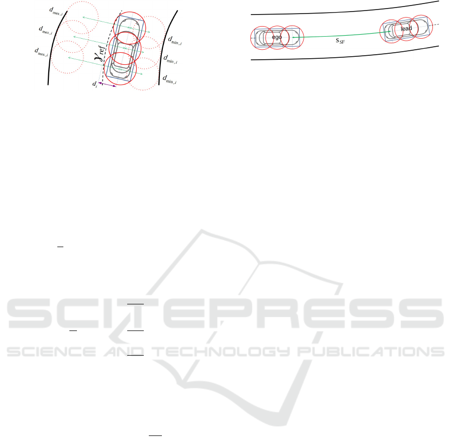
Figure 2: Representation of clearance constraints for driving
within the permissible area (clear
LN
).
by restricting the ego-vehicle’s lateral offset
d
to the
reference curve
γ
re f
as per the traffic lane markings
on the right and left sides as depicted in Figure 2. For
the lateral offset of each of the the ego-vehicle’s disks
d
i
, we define the constraints
d
min,i
≤ d
i
≤ d
max,i
,∀i ∈
{1,...,nrDisk
ego
}
, in which we calculate
d
i
of any
disk using trigonometric functions with an assumed
constant
κ
re f
across the ego-vehicle’s length
l
(Gutjahr
et al., 2017). For example, assume we have 3 disks of
constant radius
r
covering the ego-vehicle, and they
are located at
l
d
2
from each other as shown in Figure 1;
when driving in one permissible lane with
γ
re f
residing
in the middle of it, we write the constraints using the
lane width (w
LN
) as:
(d)
2
≤
w
LN
2
− r
2
(2a)
d +
l
d
2
sinχ
2
≤
w
LN
2
− r
2
(2b)
d + l
d
sinχ
2
≤
w
LN
2
− r
2
(2c)
If needed, we may use slack-variables
η
LN
≥ 0
(Britzelmeier and Gerdts, 2020) to relax the clearance
constraints, which allows for reaching a better compro-
mise between solution feasibility and system stability
(Vu et al., 2021). For example, we can write this for
the first disk as
clear
LN,1
:= (d)
2
− (
w
LN
2
− r)
2
≤ η
LN
.
2.3 Clearance Constraints for Safe
following
As defined in (Bouska, 2021), a minimum longitu-
dinal clearance (safety distance) must always be kept
between the ego-vehicle and the closest leading traffic
participant in the same lane. This can be determined
using a modified Constant Time Headway policy
(Swaroop and Rajagopal, 2001) as:
s
SF
(t) = max(s
SF,min
,v(t)t
h
)
(3)
where
s
SF,min
is the minimum safety distance,
t
h
is
the specified time headway, and
s
SF
is the required
safety distance. To enforce this metric, (Bosch, 2003)
proposes to identify the closest road user in the same
Figure 3: Required clearance for safe following (clear
SF
).
lane as the ego-vehicle and enforce the safety distance
only for this particular user, which is both simple and
valid. We achieve this by adding a clearance constraint
clear
SF
between the rearmost coverage disk of the
leading road user and the foremost disk of the ego-
vehicle as:
s
lead
− s
ego
≥ s
SF
(4)
where
s
lead/ego
represents the arc length of the leading
road user and ego-vehicle respectively. Like
clear
LN
,
clear
SF
can be relaxed with η
SF
≥ 0.
2.4 Identification of the Closest In-lane
Road User
To appropriately enforce
clear
SF
, we first need to
identify the leading in-lane road user, i.e., the closest
user driving in the same lane as the ego-vehicle. (Chen
et al., 2021) computes the probability that a road
user is in-lane using its relative lateral position and
velocity separately, then merges this information to
build a combined probability map. However, this
approach is lacking, as the analysis of the relative
lateral velocity is inherently dependent on the position.
So instead, we propose to analyze the codependent
probabilities that a road user is in-lane based on its
relative lateral position and velocity simultaneously,
then augment this data with its longitudinal distance to
get a combined probability value
P
inLN
. Here, we will
only consider the rearmost coverage disk of other road
users in the identification process for simplification.
After computing
P
inLN
for all road users, we simply
choose the user with the highest value as the leading
road user. Note that this approach not only promotes
safety by giving higher priority to road users closer
to the ego-vehicle, but it also reacts proactively to
both Cut-In and Cut-Out maneuvers, which is not
guaranteed by (Chen et al., 2021).
2.4.1 Relative Lateral Distance
The possibility that a road user exists in the same
lane as the ego-vehicle is inversely proportional to the
relative lateral deviation between them, as calculated
with respect to the reference curve
γ
re f
. We define
the probability
P
inLN,d
∈ [0, 1]
, where the road user is
considered in-lane when
P
inLN,d
= 1
and not in-lane
when
P
inLN,d
= 0
, and we derive this value from the
VEHITS 2022 - 8th International Conference on Vehicle Technology and Intelligent Transport Systems
154
relative lateral deviation
d
rel
= d
oth
− d
ego
using the
sigmoid function:
P
inLN,d
=
1
1 + e
(α
d
+β
d
|d
rel
|)
,d
rel
∈ R
(5)
where
α
d
and
β
d
are specified based on the lane width
-6 -5
-w
LN
-3
−w
LN
2
-r
ego
0
r
ego
w
LN
2
3
w
LN
5 6
0.0
0.2
0.4
0.6
0.8
1.0
d
rel
[m]
P
inLN,d
f(x) =
1
1+e
(α
d
+β
d
|d
rel
|)
Figure 4: P
inLN,d
determines in-lane road users from d
rel
.
w
LN
and the radius of the ego-vehicle’s coverage disks
r
ego
. An example of
P
inLN,d
is depicted in Figure 4
with
r
ego
= 1.0m
and
w
LN
= 4m
. Similarly, we can
define functions to calculate the probability that a user
is in the right or left adjacent lanes based on
d
rel
, which
will be useful in the next section.
2.4.2 Relative Lateral Velocity
Here, we define the probability
P
inLN,v
∈ [0, 1]
derived
from the relative lateral velocity
v
rel,y
= v
oth,y
− v
ego,y
by using sigmoid functions, but we make a distinction
between in-lane road users, i.e., whose
d
rel
is lower
than a specific threshold, and users driving in the
adjacent right/left lanes. For in-lane users,
P
inLN,v
is
inversely proportional to
v
rel,y
, as a low lateral velocity
denotes a high probability to continue driving in-lane
and a high
v
rel,y
resembles a Cut-Out maneuver. We
write this in a similar manner to Equation 5 to get the
function demonstrated in Figure 5.
−4.0 −3.0 −2.0 −1.0 0.0 1.0 2.0 3.0 4.0
0.0
0.2
0.4
0.6
0.8
1.0
v
rel,y
[m/s]
P
inLN,v
left
right
in-lane
Figure 5: Calculation of
P
inLN,v
from
v
rel,y
for in-lane road
users (blue), for users in the right lane (red) and in the left
lane (green).
Alternatively,
P
inLN,v
of road users driving in
adjacent lanes must be calculated as a combination
of both relative position and velocity. On the one hand,
if the user is driving in the right adjacent lane with a
positive
v
rel,y
, it indicates a Cut-In maneuver, i.e., a
−4
−2
0
2
4
-w
LN
-
w
LN
2
0
w
LN
2
w
LN
0
0.5
1
v
rel,y
[m/s]
d
rel
[m]
P
inLN,d,v
Figure 6: Combined probability
P
inLN,d,v
from
d
rel
and
v
rel,y
.
high probability to drive in-lane in an upcoming time
step. Likewise, a Cut-In maneuver is plausible when
the user is driving on the left with a negative
v
rel,y
. On
the other hand, when the user is driving on the right
with a negative relative velocity, it indicates a right-
hand turn maneuver, i.e.,
P
inLN,v
= 0
as the user will
not realistically be driving in-lane of the ego-vehicle.
To recap, we have three probabilities
P
inLN,d,i
,∀i ∈
{1,2,3}
, with which we identify the road user’s
location to be in-lane or in the right/left adjacent lanes.
We have also three probabilities
P
inLN,v,i
that indicate
whether the user will continue to drive in its current
lane or perform a Cut-In/Cut-Out maneuver. So, by
combining these probabilities with different weighing
factors
ω
i
as shown in Equation 6, we finally reach the
probability
P
inLN,d,v
, which represents the likelihood
a road user is in-lane of the ego-vehicle. This is also
illustrated in Figure 6.
P
inLN,d,v
=
3
∑
i=1
ω
n
· P
inLN,d,i
· P
inLN,v,i
(6)
2.4.3 Relative Longitudinal Distance
Lastly, we need to augment
P
inLN,d,v
with the user’s
relative longitudinal distance
s
rel
= s
oth
− s
ego
to
prioritize road users driving closer to the ego-vehicle
for safety considerations. In urban driving scenarios,
the ego-vehicle typically drives with a maximum
speed of
v
max
= 50[km/h]
(Bouska, 2021), for which a
corresponding safety distance can be computed using
(Swaroop and Rajagopal, 2001). Subsequently, we
define P
inLN,s
as:
P
inLN,s
=
1
1 + e
(α
s
+β
s
s
rel
)
,s
rel
∈ R
(7)
which is combined with P
inLN,d,v
to yield:
P
inLN
= P
inLN,s
· P
inLN,d,v
(8)
After calculating
P
inLN
for all road users, the user
with the highest probability is selected as the leading
Deterministic Operating Strategy for Multi-objective NMPC for Safe Autonomous Driving in Urban Traffic
155

0.0 5.0 10.0 15.0 20.0 25.0 30.0 35.0 40.0
0.0
0.5
1.0
s
rel
[m]
P
inLN,s
Figure 7: P
inLN,s
prioritizes close road users.
road user, for which
clear
SF
will be enforced. In case
multiple users have the exact same
P
inLN
, we choose
the user with the smallest
s
rel
value, prioritizing closer
users as intended. Note that with this formulation, we
may enforce
clear
SF
for a vehicle currently not in-lane
but is performing a Cut-In maneuver, which increases
the robustness of this approach and yields smoother
system controls.
2.5 System Operational Limits
When driving in urban traffic, we must adhere to the
laws and regulations, e.g., maximum/minimum speed
limits. In addition, the physical construction of the ego-
vehicle imposes restrictions on the system controls,
as there is a cap on the maximum transmitted power
by the steering actuator and the gas pedal or brakes
(Gutjahr et al., 2017). We may also include safety-
oriented constraints, such as limiting speed to avoid
excessive lateral forces when driving in sharp curves
(Gerdts, 2018), or comfort-oriented constraints, such
as limiting the rate of change of the controls (Xiao
et al., 2021). This has already been exhaustively
discussed in literature, so we summarize by saying
that the system adheres to the following constraints:
v
min
≤ v(t) ≤ v
max
(9a)
a
min
≤ a(t) ≤ a
max
(9b)
κ
min
≤ κ(t) ≤ κ
max
(9c)
u
min
≤ u(t) ≤ u
max
(9d)
and we refer the reader to (Xiao et al., 2021), (Luo
et al., 2010), and (Chen et al., 2021) for further details.
2.6 MPC Cost Function Formulation
In this part, we focus on modeling the different goals in
the multi-objective MPC cost function. We start with
trajectory tracking, where our objective is to follow
a desired path that spans from a start location
A
to a
destination
B
, such that this path can be modeled as
a spline curve
γ
re f
: [s
0
,s
f
] → R
2
with the way-points
γ
re f
(s) := [x
re f
(s),y
re f
(s)]
T
. We deliberately chose
the dynamical model in Equation 1 to represent the
ego-vehicle’s movement with respect to a reference
trajectory, as there exists a subset of the system states
that mirrors tracking errors to this trajectory. In other
words, for the system states vector
x(t) ∈ R
n
x
, we have
the error states vector
y(t) ∈ R
n
y
with
n
x
≥ n
y
, and the
path tracking problem is equivalent to stabilizing
y(t)
to
0
(Xiao et al., 2021). Additionally, we model the
incentive to reach the destination
B
as minimizing the
difference between
s
and the total traveled distance at
the destination
s
f
, or rather normalize it as
s
f
−s
s
f
−s
0
for
more consistent results.
Second, we employ a typical objective to improve
passenger comfort and reduce fuel consumption, i.e.,
minimizing the system controls vector
u(t) ∈ R
n
u
(Luo et al., 2010). Finally, we include any added
slack variables for constraints relaxation, such as
η
LN,i
,i ∈ {1, ...,n
LN
}
for admissible driving
clear
LN
,
and, if a leading in-lane road user exists,
η
SF
for
safe following. This yields the combined cost function:
min
Z
T
0
ω
y
||y|| +ω
s
s
f
− s
s
f
− s
0
2
+ω
u
||u||+
n
LN
∑
i=1
ω
LN
η
LN,i
2
+ ω
SF
η
SF
2
dt
(10)
with the weighing factors
ω
y
for path tracking,
ω
s
for
maximizing travel distance,
ω
u
for minimizing control
effort, and
ω
LN/SF
for relaxing the different clearance
constraints. Note that this cost function is subject to
the system dynamics (1), the operational limits (9) and
the relaxed clearance constraints:
clear
LN,i
≤ η
LN,i
,∀i ∈ {1,...,n
LN
}
clear
SF
≤ η
SF
,O
inLN
6=
/
0,O
inLN
∈ O
oth
(11)
where
O
oth
is the set containing all other road users
and
O
inLN
is a single-entry set that contains the leading
in-lane road user. This function serves as a basis for all
controllers we intend to develop, as we can fine-tune
the different
ω
factors for specific driving scenarios
to better achieve their corresponding objectives, e.g.,
by prioritizing collision avoidance to path tracking in
case of approaching a stationary object.
3 URBAN DRIVING AND
VEHICLE CONTROL
To construct the system controller, we revise various
sources that describe what a typical urban driving
scenario entails, such as (Yurtsever et al., 2020),
(Bae et al., 2020), and (Bosch, 2003). We also
employ sources like (Bouska, 2021) and (ISO Central
Secretary, 2018) to develop performance tests, with
which we can guarantee the system credibility. In
general, the ego-vehicle must travel across
[s
0
,s
f
]
VEHITS 2022 - 8th International Conference on Vehicle Technology and Intelligent Transport Systems
156

while adhering to the driving regulations and, when
other road users exist, it must correctly identify the
leading in-lane user and follow it at a safe distance to
avoid collisions. Furthermore, it must adequately react
to situations like Cut-In/Cut-Out maneuvers and traffic
jams (Automatic Stop maneuver), and operate reliably
both in straight and curved trajectories. Accordingly,
we define four major sequences (Exit Parking, Path
Following, Pulling Up, and Enter Parking), such that
during a typical scenario, the ego-vehicle is either in
one of these sequences or transitioning from one to the
other. For each sequence, we develop and fine-tune
a NMPC-based controller (with calibrated objectives
and constraints), and we introduce a FSM to activate
and switch between the different sequences and their
corresponding controllers. This will be discussed in
detail in the upcoming paragraphs.
3.1 FSM Architectural Approach
The FSM model is one of the fundamental methods for
designing rule-based controllers (Macedo et al., 2015).
From a mathematical perspective, it is a deterministic
model of computation that portrays a system using
states (also known as modes), inputs, and transition
dynamics, and can be expressed as a quintuple
M :=
(S,Σ, δ,S
0
,F)
, where
S
is the finite (non-empty) set
of states with
S
0
∈ S
as the initial state,
Σ
is the finite
(non-empty) set of inputs,
δ : S × Σ → S
represents the
inter-state transition function, and
F ⊆ S
is the set of
final states. For its operation, the FSM starts in
S
0
and,
according to the system input
σ
and transition function
δ
, it makes a transition to a different state
f ∈ S
. Then,
f
is set as
S
0
and possible transitions are checked for
the new
σ
and
δ
; this process is repeated until the final
state is reached, for which
F
is an empty set (or is
endlessly repeated if the FSM is cyclic) (Klose and
Mester, 2018).
Exit
Parking
(XP)
Path
Following
(PF)
Pulling
Up
(PU)
Standstill
(SS)
Enter
Parking
(NP)
End
(ND)
τ
1
τ
2
τ
3
τ
2
τ
4
τ
5
τ
6
τ
7
Figure 8: Configuration of the FSM modes and their possible
transitions.
The FSM depicted in Figure 8 incorporates the
aforementioned driving sequences, with the addition
Table 1: FSM mode switch conditions.
S
0
f
XP PF PU NP SS ND
XP OW τ
1
- - - -
PF - OW τ
3
τ
2
- -
PU - τ
4
OW τ
2
τ
5
-
SS - - - τ
6
OW -
NP - - - OW - τ
7
of the state (Standstill), which gets activated when the
ego-vehicle drives with a very slow speed
v ≤ 0.5[m/s]
to avoid infeasible and aggressive system controls,
and the final state (End ) which promptly stops the
ego-vehicle upon reaching its destination. Also, the
conditions for switching between the FSM modes are
portrayed in Table 1 with the symbols
τ
i
, such that a
currently active state remains unchanged when all of
its exit conditions are not satisfied (denoted with OW).
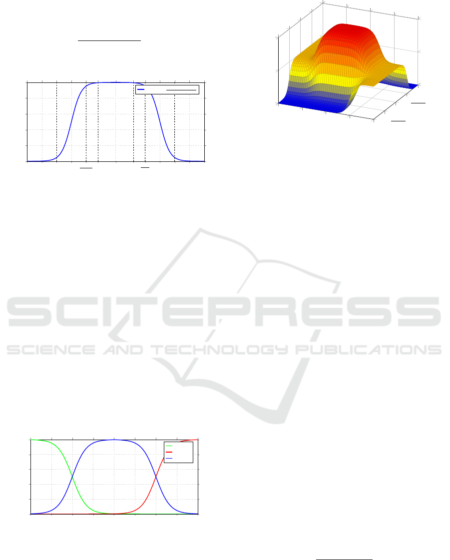
Exit Parking (XP).
This is the initial state that gets
activated when starting the trip at
A
and it denotes that
the ego-vehicle is currently driving inside the parking
area. This imposes a restriction on the maximum speed
(no faster than walking speed) and allows for sharper
turns (due to traveling slowly), and, accordingly, we
can calibrate the system constraints (cf. Equation
9) and objectives (cf. Equation 10). Since we
already have
γ
re f
in accordance with geographical
data, we can detect whether the ego-vehicle is inside
the parking area or not by comparing
s
to a threshold
s
XP
, such that the condition for leaving the parking
area
τ
1
is fulfilled when
s ≥ s
XP
. However, this yields
aggressive controls, so we replace the hard equality
condition with a transitioning phase between
s
XP
and
a relaxed threshold
s
XP,η
. Consequently, we compute
a transitioning factor
ω
τ
1
from
s
XP
and
s
XP,η
as shown
in Figure 9, and we revise τ
1
to be:
(s ≥ s
XP,η
→ τ
1
= 1) ∧ (s < s
XP,η
→ τ
1
= 0)
(12)
where
τ
1
is only fulfilled after passing the transitioning
phase threshold s
XP,η
.
s
0
s
XP
s
XP,η
0.0
0.2
0.4
0.6
0.8
1.0
s[m]
ω
τ
1
Figure 9:
ω
τ
1
yields smooth controls when transitioning
from XP to PF.
Initially, we attempted to compute the transitioning
Deterministic Operating Strategy for Multi-objective NMPC for Safe Autonomous Driving in Urban Traffic
157

control action as a weighted average of the two state
controllers with
u
τ
1
= ω
τ
1
· u
XP
+ (1 −ω
τ
1
) · u
PF
. Yet,
this yielded a sub-optimal
u
τ
1
, despite both
u
XP
and
u
PF
being optimal. Alternatively, we attain optimal
controls during the transitioning phase by introducing
a new problem, at which
ω
τ
1
gradually modifies the
system objectives and constraints. For example, we
adjust the objective for path following to be:
ω
y,τ
1
= ω
y,XP
+ (ω
y,PF
− ω
y,XP
) · (1 − ω
τ
1
)
(13)
which is similarly done for all other objectives. As
for the system constraints, we have no problem when
transitioning to a less restricted environment, e.g.,
when
v
max,XP
≤ v
max,PF
, as the constraint
v ≤ v
max,PF
is already fulfilled, so we use the same approach
as Equation 13. Nevertheless, this is invalid when
κ
max,XP
≥ κ
max,PF
, as an optimal control may already
be at the operational limit
κ = κ
max,XP
, yielding an
infeasible problem with
κ κ
max,PF
. Instead, we relax
this constraint (and all other similar cases) using:
κ
max,τ
1
= κ
max,XP
+ (κ
max,PF
− κ
max,XP
) · (1 − ω
τ
1
),
κ − κ
max,τ
1
≤ η
κ
max
(14)
thus we have a feasible control problem that can be
optimally solved to achieve a smooth state transition.
Path Following (PF).
This is the core urban driving
sequence, where the ego-vehicle travels with an
admissible speed and tries to maximize the traveled
distance to its destination. Here, the turning curvature
is restricted more than XP to avoid excessive lateral
forces when turning with high speeds (promotes safety
and comfort), and similarly for acceleration. There
are multiple exit transitions from PF, thus we need
to define a priority, or rather an order of operations
(Zhang et al., 2017), with which we can sequentially
evaluate these transitions. We specify the transition
τ
2
to NP as the highest priority condition, as it implies
that we are close to our destination
B
. Similar to
τ
1
,
we use geo-data to determine a threshold
s
NP
based
on
s
f
, and add a transitioning phase between a relaxed
threshold
s
NP,η
and
s
NP
using the transitioning factor
ω
τ
2
, with:
(s ≥ s
NP
→ τ
2
= 1) ∧ (s < s
NP
→ τ
2
= 0)
(15)
The transition
τ
3
to PU denotes that the ego-vehicle
travels much slower than the speed limit either due to
following a slow leading road user or approaching a
traffic jam. So, we use the speed limits to construct the
transitioning factor ω
τ
3
as shown in Figure 11, with:
τ
3
:= ¬τ
2
∧
v ≤
v
max
− v
min
2
∧ (O
inLN
6=
/
0)
(16)
s
NP,η
s
NP
s
f
0.0
0.2
0.4
0.6
0.8
1.0
s[m]
ω
τ
2
Figure 10: ω
τ
2
for transitioning from PF to NP.
v
max
−v
min
2
v
max
−v
min
1.2
0.0
0.2
0.4
0.6
0.8
1.0
v[m/s]
ω
τ
3
Figure 11: ω
τ
3
for transitioning from PF to PU.
Pulling Up (PU).
This sequence is not only suitable
for following slow road users or approaching stationary
ones, but can also be used for stopping at traffic lights
by modeling the traffic junction as a stationary leading
road user. Here, we prioritize
ω
SF
compared to
ω
s
to
guarantee safety, and likewise adapt other objectives’
weights. We also allow for more aggressive controls
due to traveling relatively slowly. Similar to PF, the
transition
τ
2
to NP has the highest priority and follows
the formula in Equation 15 with the same transitioning
factor
ω
τ
2
. Afterwards, we have the transition
τ
4
to
PF, which has a higher priority than the transition
τ
5
to SS to discourage the system from performing a
complete stop when a stationary leading road user
starts to accelerate. Complementary to Equation 16,
we construct the transition phase elements as:
τ
4
:= ¬τ
2
∧
v ≥
v
max
− v
min
1.2
∨ (O
inLN
=
/
0)
,
ω
τ
4
= 1 − ω
τ
3
(17)
Standstill (SS).
Next, we have the utility state SS,
which is responsible for completely stopping the ego-
vehicle behind a stationary object, and acts as a buffer
that prevents needless start-stop maneuvers behind a
very slow leading user. First, we have the transition
τ
5
from PU to SS, which we define as:
τ
5
:= ¬τ
4
∧ (v ≤ 0.5[m/s]) ∧ (a ≤ 0[m/s
2
])
(18)
and implement as a hard constraint, which is accept-
able at this speed. This transition promptly stops the
ego-vehicle if it is traveling very slowly while deceler-
ating. Next, we have the transition
τ
6
from SS back to
PU, which we compute from the relative distance to
VEHITS 2022 - 8th International Conference on Vehicle Technology and Intelligent Transport Systems
158
the leading user
s
rel
= s
lead
− s
ego
, the required safety
distance s
SF
, and an additional threshold s
SF,η
by:
τ
6
:= (s
rel
≥ s
SF
+ s
SF,η
) ∨ (O
inLN
=
/
0)
(19)
which will either be fulfilled when the leading user
starts moving (and cover a certain distance), or when
no leading user can be detected anymore (relevant for
modeling traffic lights).
Enter Parking (NP).
This state is very similar to XP,
with one difference being that we are almost at our
destination. So, we have only one transition
τ
7
to the
final state ND, which we calculate from
s
,
s
f
, and
some threshold s
ND
as:
(s
f
− s ≤ s
ND
→ τ
7
= 1) ∧ (s
f
− s > s
ND
→ τ
7
= 0)
(20)
such that when
τ
7
is fulfilled, we directly transit to
ND and promptly decelerate the ego-vehicle until a
complete stop, thus concluding our trip.
Finally, it is worth mentioning that the proposed
FSM architecture is loosely coupled with the NMPC
strategy implemented in this work, i.e., we can make
slight adaptations and employ this architecture for
other control techniques as well, which may be
investigated in future work.
4 NUMERICAL SIMULATION
AND RESULTS
The proposed control architecture is implemented
entirely in Fortran and the software OCPID-DAE1 is
used to solve the formulated optimal control problem.
To adequately evaluate the developed controller, we
designed two test scenarios that combine different
maneuvers, e.g., Cut-In and Cut-Out, as well as require
transitioning between the different FSM states.
Figure 12: Travel path for the first test.
The first scenario includes a full test run from start
to finish, where the ego-vehicle follows a trajectory
with different turns and attempts to reach its destina-
tion as fast as possible. The travel path is shown in
Figure 12, such that the ego-vehicle traverses this path
with minimal error as illustrated in Figure 13. More-
over, the ego-vehicle travels with the speed trajectory
Figure 13: Tracking error states for the first test.
depicted in Figure 14, which denotes a smooth trajec-
tory with comfortable acceleration and deceleration.
Finally, the currently active FSM state and state transi-
tions are demonstrated in Figure 15.
Figure 14: Speed trajectory for the first test.
Figure 15: Active FSM states for the first test.
The second test focuses on evaluating the system
performance with multiple road users, while the
ego-vehicle is traversing a straight line trajectory.
Moreover, this scenario directly starts in the PF state
for simplification. Initially, the ego-vehicle is traveling
with
v = 13.5[m/s]
, and we have two users in the
scenario: one in-lane at
s
rel,o1
= 41[m]
, and the other
in the left lane at
s
rel,o2
= 36[m]
, such that they both
travel with
v = 12[m/s]
. In the first few seconds,
the ego-vehicle continues to travel with its initial
speed as
s
rel
> s
SF
, but as it approaches the in-lane
vehicle, it decelerates to match its velocity of
12[m/s]
as illustrated in Figure 16.
At
t = 16[s]
, the vehicle in the left lane performs
a Cut-In maneuver to the driving lane, and the ego-
vehicle decelerates to maintain the safety distance
s
SF
,
then accelerates afterwards to match the speed
v
o2
of
the new in-lane leader. Around
t = 34[s]
, this user
starts to decelerate and the ego-vehicle decreases its
speed to match
v
o2
until the user performs a Cut-Out
maneuver around
t = 40[s]
, at which the ego-vehicle
Deterministic Operating Strategy for Multi-objective NMPC for Safe Autonomous Driving in Urban Traffic
159
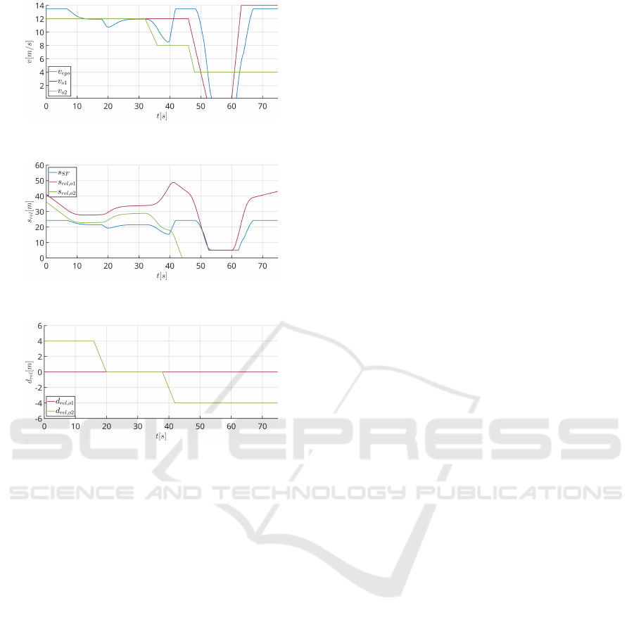
Figure 16: Speed trajectories of all road users in the second
test.
Figure 17: Safety distance
s
SF
is kept to the leading in-lane
road user during the second test.
Figure 18: d
rel
of other road users in the second test.
accelerates till it reaches the maximum allowed speed.
Finally, we test a Closing maneuver as the ego-vehicle
recognizes a stationary object in-lane at
t = 48[s]
and
appropriately decelerates until it reaches a complete
stop at
t = 54[s]
. The ego-vehicle remains stationary
until the leading in-lane road user has passed the
relaxed safety distance
s
rel
>= s
SF
+s
SF,η
, after which
it starts moving again and accelerates appropriately
until it reaches its maximum allowed speed, thus
concluding our numerical experiments.
5 CONCLUSION AND FUTURE
WORK
In this work, we introduced a FSM architectural model
for operating multiple multi-objective NMPC-based
controllers in urban driving scenarios. We simu-
lated our approach and successfully tested it against
different scenarios, proving its effectiveness in gener-
ating smooth control trajectories, while minimizing
the path tracking errors and the overall travel time.
Moreover, we integrated a probabilistic approach to
determine the closest in-lane leading road user, with
which we enforced collision avoidance constraints to
guarantee the ego-vehicle’s safety.
For future work, we may investigate a more
generic approach for tuning the weighing factors of
the different objectives in the MPC multi-objective
cost function, e.g., using machine learning. We may
also extend the path tracking problem so as to enable
overtaking of slower vehicles, for which new FSM
states and transitions will be necessary. Finally, we
may formulate our problem using a Mixed-Integer
Programming (MIP) approach then validate it using
the same test scenarios, such that we can comparatively
evaluate the FSM and MIP methodologies in terms
of robustness, computational complexity, and overall
performance.
ACKNOWLEDGEMENTS
This research paper is funded by dtec.bw – Digi-
talization and Technology Research Center of the
Bundeswehr as part of project MORE – Munich
Mobility Research Campus.
REFERENCES
Bae, S.-H., Joo, S.-H., Pyo, J.-W., Yoon, J.-S., Lee, K., and
Kuc, T.-Y. (2020). Finite state machine based vehicle
system for autonomous driving in urban environments.
In 2020 20th International Conference on Control,
Automation and Systems (ICCAS), pages 1181–1186.
Bosch, R. (2003). ACC Adaptive Cruise Control. Bentley
Pub.
Bouska, W. (2021). StVO Straßenverkehrs-Ordnung. C.F.
M
¨
uller.
Britzelmeier, A. and Gerdts, M. (2020). A nonsmooth
newton method for linear model-predictive control
in tracking tasks for a mobile robot with obstacle
avoidance. IEEE Control Systems Letters, PP:1–1.
Britzelmeier, A., Gerdts, M., and Rottmann, T. (2020).
Control of interacting vehicles using model-predictive
control, generalized nash equilibrium problems, and
dynamic inversion. IFAC-PapersOnLine, 53(2):15146–
15153. 21st IFAC World Congress.
Burger, M. and Gerdts, M. (2019). DAE Aspects in Vehicle
Dynamics and Mobile Robotics, pages 37–80. Springer
International Publishing, Cham.
Chen, C., Guo, J., Guo, C., Chen, C., Zhang, Y., and Wang,
J. (2021). Adaptive cruise control for cut-in scenarios
based on model predictive control algorithm. Applied
Sciences, 11(11):5293.
Gerdts, M. (2018). Numerical experiments with multistep
model-predictive control approaches and sensitivity
updates for the tracking control of cars.
Gr
¨
une, L. and Pannek, J. (2011). Nonlinear Model Predictive
Control: Theory and Algorithms. Springer London Ltd.
VEHITS 2022 - 8th International Conference on Vehicle Technology and Intelligent Transport Systems
160

Gutjahr, B., Gr
¨
oll, L., and Werling, M. (2017). Lateral
vehicle trajectory optimization using constrained linear
time-varying mpc. IEEE Transactions on Intelligent
Transportation Systems, 18(6):1586–1595.
ISO Central Secretary (2018). Intelligent transport systems
— Adaptive cruise control systems — Performance
requirements and test procedures. Standard, Interna-
tional Organization for Standardization, Geneva, CH.
Klose, P. and Mester, R. (2018). Simulated autonomous
driving in a realistic driving environment using deep
reinforcement learning and a deterministic finite state
machine. CoRR, abs/1811.07868.
Lu, M., Wevers, K., van der Heijden, R., and Heijer, T.
(2004). Adas applications for improving traffic safety.
In 2004 IEEE International Conference on Systems,
Man and Cybernetics (IEEE Cat. No.04CH37583),
volume 4, pages 3995–4002 vol.4.
Luo, L., Liu, H., Li, P., and Wang, H. (2010). Model predic-
tive control for adaptive cruise control with multi-
objectives: Comfort, fuel-economy, safety and car-
following. Journal of Zhejiang University SCIENCE
A, 11:191–201.
Macedo, B. H. F., Araujo, G. F. P., Silva, G. S., Crestani,
M. C., Galli, Y. B., and Ramos, G. N. (2015).
Evolving finite-state machines controllers for the
simulated car racing championship. In 2015 14th
Brazilian Symposium on Computer Games and Digital
Entertainment (SBGames), pages 160–172.
Studier, R. (2022). Straßenverkehrs-Zulassungs-Ordnung
StVZO. Epubli.
Swaroop, D. and Rajagopal, K. (2001). A review of constant
time headway policy for automatic vehicle following.
In ITSC 2001. 2001 IEEE Intelligent Transportation
Systems. Proceedings (Cat. No.01TH8585), pages 65–
69.
Vu, T. M., Moezzi, R., Cyrus, J., and Hlava, J. (2021). Model
predictive control for autonomous driving vehicles.
Electronics, 10(21):2593.
Xiao, W., Mehdipour, N., Collin, A., Bin-Nun, A. Y., Fraz-
zoli, E., Tebbens, R. J. D., and Belta, C. (2021). Rule-
based evaluation and optimal control for autonomous
driving. CoRR, abs/2107.07460.
Yurtsever, E., Lambert, J., Carballo, A., and Takeda, K.
(2020). A survey of autonomous driving: Common
practices and emerging technologies. IEEE Access,
8:58443–58469.
Zhang, M., Li, N., Girard, A., and Kolmanovsky, I. (2017). A
finite state machine based automated driving controller
and its stochastic optimization. volume Volume 2:
Mechatronics; Estimation and Identification; Uncertain
Systems and Robustness; Path Planning and Motion
Control; Tracking Control Systems; Multi-Agent and
Networked Systems; Manufacturing; Intelligent Trans-
portation and Vehicles; Sensors and Actuators; Diag-
nostics and Detection; Unmanned, Ground and Surface
Robotics; Motion and Vibration Control Applications
of Dynamic Systems and Control Conference.
Deterministic Operating Strategy for Multi-objective NMPC for Safe Autonomous Driving in Urban Traffic
161
