Persistent Homology based Classiﬁcation of Chaotic Multi-variate Time

Series with Application to EEG Data

Martina Flammer and Knut H

uper

Institute of Mathematics, Julius-Maximilians-Universit

at W

urzburg, Emil-Fischer-Straße 31, W

urzburg, Germany

Keywords:

Bottleneck Distance, Dimension Reduction, Dynamical Component Analysis, Persistent Homology,

Simplicial Complex, Topological Data Analysis.

Abstract:

An application of persistent homology for detection of epileptic events in EEG data is presented. Given

point cloud data, persistent homology is a tool from topological data analysis to describe the structure of the

underlying space on which the data was sampled by utilizing topological invariants and tracking their behavior

on several spatial scales. As a preprocessing step, a novel method called Dynamical Component Analysis is

used that reduces the dimension of a multi-variate time series by incorporating information about the dynamics

of the system. The results show that our proposed method is appropriate to detect the occurence of petit-mal

epileptic seizures in EEG signals.

1 INTRODUCTION

According to the WHO, almost 50 million people suf-

fer under epilepsy, which makes it one of the most

frequent neurological diseases. Being unable to cure

epilepsy, patients are usually dependent on medica-

tion, making the detection and forecast of epilep-

tic events a particularly important task that is com-

monly accomplished by measuring brain activity us-

ing an electroencephalogram (EEG). These data are

measured by placing electrodes on the scalp of pa-

tients that measure the summed electrical brain activ-

ity. However, even for experts it can be difﬁcult and

time-consuming to classify EEG data of every single

patient, which makes the automated classiﬁcation and

interpretation of EEG data a tremendous challenge for

data scientists from various ﬁelds, in particular, from

a mathematical and an engineering point of view.

Since it is assumed that during epileptic events the

activity of neurons is more synchronized, we believe

that the EEG data set is revealing some mathemati-

cal structure that is the key ingredient to classify EEG

data with respect to seizure and non-seizure activ-

ity. Such an assumption follows the paper (van Veen

and Liley, 2006) where Shilnikov chaos was proposed

during epileptic events.

Being on the intersection of topology, the tradi-

tional mathematical ﬁeld that investigates structures,

and data science, topological data analysis seems to

be an appropriate approach to the above mentioned

task. Especially its main method, persistent homol-

ogy, is considered here as a procedure to describe the

structure of spaces on which data was sampled. Basi-

cally, it uses tools from computational topology com-

bined with geometric insight to provide connectivity

information of the underlying space on several spa-

tial scales. Having its theoretical fundaments in alge-

braic topology leads to a well-understood foundation

of persistent homology. Further advantages are that

the method is robust with respect to small perturba-

tions of the input data and is able to cope with com-

plex data sets, making it particularly useful for analy-

sis of big data. Since the original formulation of per-

sistent homology in the early 2000s, a lot of research

is going on in order to extend the ﬁeld in various di-

rections and to complete the framework.

Although persistent homology is able to process

high-dimensional data sets it still requires a lot of

computational time. To circumvent this drawback

we preprocess the data using Dynamical Component

Analysis (DyCA) (Uhl et al., 2020), a novel method

to reduce the dimension of a time series by regarding

the dynamics of the underlying system. It can be ap-

plied whenever the dynamics is modeled by a system

of ordinary differential equations (ODEs) with linear

as well as non-linear equations, which is the case for

EEG data (Friedrich and Uhl, 1996).

The outline of this paper is the following. In Sec-

tion 2, the preprocessing of the data with DyCA is

described. Section 3 will focus on the mathematical

Flammer, M. and Hüper, K.

Persistent Homology based Classiﬁcation of Chaotic Multi-variate Time Series with Application to EEG Data.

DOI: 10.5220/0011144800003271

In Proceedings of the 19th International Conference on Informatics in Control, Automation and Robotics (ICINCO 2022), pages 595-604

ISBN: 978-989-758-585-2; ISSN: 2184-2809

595

description of persistent homology, from its algebraic

basics to its application to point cloud data and its vi-

sualization. In Section 4, the EEG data sets are speci-

ﬁed that are used to test out proposed approach. Sec-

tion 5 is devoted to the description of the exact proce-

dure in our numerical experiments and the presenta-

tion of the results, which is followed by an outlook to

future work in Section 6.

2 PREPROCESSING

In (Uhl et al., 2020), the authors introduced a novel

method for dimensionality reduction and separating

the deterministic part of the data from the stochastic

part that corresponds to the noise components. This

method, called DyCA, can be applied to multivariate

time-series if the underlying model for the dynam-

ics follows a system of ODEs which consists of lin-

ear as well as non-linear equations. Using the lin-

ear part, amplitudes and multivariate modes are de-

termined that ﬁt the system of ODEs optimally. This

task is accomplished by solving a generalized eigen-

value problem that is derived from a least squares

minimization problem. The eigenvalue problem leads

to a collection of eigenvalues and associated eigen-

vectors together with some corresponding vectors v

which both together form the set of projection vec-

tors. Eigenvalues close to 1 correspond to modes for

which the linear approximation ﬁts well. Introduc-

ing a threshold for the eigenvalues allows to estimate

the number of linearly coupled components. Further-

more, also the total number of equations n, governed

by the ODE system, is estimated as being the dimen-

sion of the span of the projection vectors. The set of

eigenvectors u

is completed by suitable v

, where the

are the projection vectors corresponding to the non-

linear equations, to a basis of R

, the relevant sub-

space. Using the projection vectors, one can project

the initial multivariate time series onto the relevant

subspace, which results in the estimated amplitudes.

The last step is again solving a least squares prob-

lem in order to obtain the pseudoinverse of the pro-

jection matrix and therefore get an estimate for the

DyCA components. In the end, the time-varying sig-

nal is reconstructed as a linear combination of the

estimated time-varying amplitudes and the estimated

DyCA components. The derivation can be found in

detail in the paper (Uhl et al., 2020).

The authors of (Uhl et al., 2020) thought of sev-

eral ways to utilize DyCA, for example for using the

eigenvalue spectrum to classify the dynamics of the

time series, for eliminating noise components of the

signal or for modeling the signal by an data-driven

approach. In our paper, we use it as a preprocess-

ing step for the projection of the given data onto a

lower-dimensional subspace and for incidentally re-

ducing the noise.

3 PERSISTENT HOMOLOGY

Persistent homology is a central topic in the ﬁeld of

topological data analysis. In topological data analy-

sis, one frequently faces the problem that a set of data

is given that was sampled on a space but the struc-

ture of the space is unknown. Persistent homology

provides a tool which allows to study the topolog-

ical invariants of this space by building a sequence

of simplicial complexes from the data, also known as

the persistence complex. By regarding several scales,

which is accomplished by tracking the topology of the

data set when the point cloud is thickened, one gets

information about connectivity of the space, such as

connected components, holes, voids, etc., which can

be used for example for the analysis of networks, dy-

namical systems and protein structures. A detailed

overview can be found in (Otter et al., 2017).

3.1 From Data to Simplicial Complexes

The ﬁrst step in the pipeline of the computation of per-

sistent homology consists of constructing a simplicial

complex from the given point cloud data. A simplicial

complex is a way to approximate a topological space

by a set of vertices, edges, triangles, tetrahedrons and

higher-dimensional equivalents. Such an approxima-

tion is called a triangulation of the space, however,

not every space is triangulable, but in our application

the assumption of triangulable spaces is appropriate.

Deﬁnition 3.1 (Simplicial complex). A simplicial

complex K is a set consisting of non-empty subsets of

a set K

such that the following two properties hold:

1. {v} ∈ K for all v ∈ K

and

2. τ ∈ K for all τ ⊂ σ,σ ∈ K.

The elements of K are called simplices and ele-

ments of K

are referred to as vertices of K. A simplex

is called p-simplex or equivalently, is said to have di-

mension p, if its cardinality is p+1. The dimension of

the simplicial complex K is deﬁned as the maximum

of dimensions of all its simplices.

A simplex τ is called a face of a simplex σ if τ ⊂ σ.

τ is called a face of σ of codimension k if the di-

mensions of τ and σ differ by k. For two simplicial

complexes K and L, a map of simplicial complexes

f : K → L is a map on the corresponding vertex sets

ICINCO 2022 - 19th International Conference on Informatics in Control, Automation and Robotics

596

f : K

→ L

with the property that simplices in K are

mapped to simplices in L, i.e. f (σ) ∈ L for all σ ∈ K.

Figure 1: Example of a simplicial complex.

In Figure 1, an example of a three dimensional

simplicial complex is shown. It consists of 0-

simplices (points), of 1-simplices (edges between

points), of 2-simplices (triangles) and of one 3-

simplex (the tetrahedron).

Given data in form of a ﬁnite point cloud, there

are several ways to construct a simplicial complex of

that data set. One of the most important complexes is

the so-called

Cech complex.

Deﬁnition 3.2. For a ﬁnite point set M in a metric

space X and some ε > 0, consider the non-empty

union M

x∈M

B(x,ε), where B(x, ε) denotes the

closed ball centered at x and with radius ε. Let

C(M,ε) be the simplicial complex with vertex set M

and where a k-simplex {x

,...,x

} ⊂ M is added to the

simplicial complex

C(M,ε) if and only if B(x

,ε) ∩

... ∩ B(x

,ε) 6=

C(M,ε) is called the

Cech complex

on M at scale ε.

An example of a

Cech complex at a certain scale ε

is shown in Figure 2. The black dots denote the point

cloud data set and the orange balls are the closed balls

around each data point. As one can see in the Figure,

an edge between two points is added to the simplicial

complex if the intersection of the two associated balls

is non-empty. In a analogue manner, triangles, tetra-

hedrons and higher-dimensional simplices are added.

Theoretically, the dimension of the

Cech complex

might become very large, namely up to |M| − 1. Ad-

ditionally, in order to check whether a subset of M is

actually a simplex, one has to check the above condi-

tion for a large number of intersections. This makes

the calculation of the

Cech complex computationally

expensive. A way to overcome these difﬁculties is by

regarding the lazy version of this simplicial complex.

That means that one only checks for pairwise inter-

sections, i.e. a simplex {x

,...,x

} is added to the sim-

plicial complex if and only if the pairwise intersec-

tions B(x

,ε) ∩ B(x

,ε) are non-empty for all indices

1 ≤ i < j ≤ k. We call this simplicial complex the

Figure 2: Example of a

Cech complex.

Vietoris-Rips complex of M at scale ε. The Vietoris-

Rips complex still can have a very large dimension,

but it is computationally cheaper, making it one of the

most popular choices for building a simplicial com-

plex on point cloud data.

3.2 Simplicial Homology

Homology is a way of classifying topological spaces.

The idea behind homology is to distinguish spaces

by their n-dimensional holes, for every n ∈ N

. 0-

dimensional holes correspond to connected compo-

nents, 1-dimensional holes to holes in the usual sense,

2-dimensional holes to voids, and so on. The homol-

ogy of a simplicial complex is constructed as follows:

Let C

(K) be the vector space over F

with basis

consisting of the p-simplices of K. Now, we deﬁne

linear maps d

on the basis elements for every p ∈

{1,2,...} as follows:

: C

(K) → C

p−1

(K),

σ 7→

∑

τ⊂σ,τ∈K

p−1

(1)

and for p = 0, let d

be the zero map. Here and in

the following, let K

denote the set of all p-simplices.

If the dimension of the simplicial complex K is n,

then the set of p-simplices K

is empty for all p > n.

Hence, the corresponding vector space C

(K) is the

zero vector space. As a consequence, the following

sequence of vector spaces and F

-linear mappings is

obtained:

n+1

−→C

(K)

−→···

−→C

(K)

−→C

(K)

−→0, (2)

which is also called a chain complex. The maps d

are referred to as boundary maps and by simple cal-

culations it follows that they have the property

◦ d

p+1

= 0 for all p ∈ {0,1,2,...}. (3)

Persistent Homology based Classiﬁcation of Chaotic Multi-variate Time Series with Application to EEG Data

597

As a consequence, im d

p+1

⊂ kerd

. This condition

allows us to consider the quotient of the two vector

spaces kerd

and imd

p+1

Deﬁnition 3.3. For any p ∈ {0, 1,2,...}, deﬁne Z

kerd

and B

:= im d

p+1

. The elements of B

are re-

ferred to as p-boundaries and the elements of Z

are

called p-cycles. Then, the quotient vector space

(K) := Z

(4)

is called the p-th homology of a simplicial complex

K. The p-th Betti number of the simplicial complex

K is deﬁned as the dimension of the p-th homology

vector space,

(K) := dim H

(K) = dim Z

− dim B

. (5)

One property of homology is that maps between

simplicial complexes f : K → L induce linear maps

between the corresponding homology vector spaces

: H

(K) → H

(L) for all p. Another important

property is functoriality: given maps of simplicial

complexes f : K → L and g : L → M, for the map-

ping (g◦ f )

: H

(K) → H

(M) it holds that (g◦ f )

◦ f

3.3 Filtrations

A sequence of nested subcomplexes of a simplicial

complex K

0 = K

⊂ K

⊂ ··· ⊂ K

= K (6)

is called a ﬁltration of K. Considering the homology

of each of the subcomplexes, for every i ≤ j the in-

clusion maps from K

to K

induce linear maps

i, j

: H

) → H

) (7)

for all p. Consequently, we also obtain for each di-

mension p a sequence of homology spaces

0=H

)→H

)→··· → H

)=H

(K) (8)

where the arrows between subsequent vector spaces

) and H

i+1

) are the above deﬁned maps

i,i+1

. Due to the already mentioned functoriality

condition it holds:

j,k

◦ f

i, j

= f

i,k

, for all i ≤ j ≤ k. (9)

Deﬁnition 3.4 (p-th persistent homology). Consider

a ﬁltration of a simplicial complex K

⊂ K

⊂ ·· · ⊂

= K. Then, the p-th persistent homology of K is

deﬁned as

i, j

:= im f

i, j

= Z

)/(B

) ∩ Z

)), (10)

where f

i, j

: H

) → H

) are the linear maps in-

duced by the inclusions maps K

→ K

for all i, j with

0 ≤ i ≤ j ≤ l.

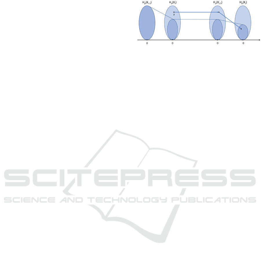
Figure 3: Class γ is born at ﬁltration step i and dies entering

ﬁltration step j, inspired by (Edelsbrunner and Harer, 2010).

Deﬁnition 3.5. A homology class γ ∈ H

) is said

to be born at ﬁltration step i if ( f

i−1,i

)

−1

(γ) =

0, i.e. it

does not lie in the image of f

i−1,i

. Intuitively, it means

that i is the smallest index on which the class appears.

Further, we say that a class γ ∈ H

) dies entering

if it merges with an older class as we go from K

j−1

to K

, that is, f

i, j−1

(γ) 6∈ H

i−1, j−1

but f

i, j

(γ) ∈ H

i−1, j

In the literature, this is referred to as elder rule.

The main idea of persistent homology is to track

the lifetime of homology classes, i.e. when classes

are born and when they die. Classes that persist on

a large scale are regarded as actual features whereas

classes with only a short lifetime are said to be caused

by noise. A way to visualize this is through a set of

intervals of the form [b

), where each interval cor-

responds to a class γ

with birth time b

and death time

. If a class with birth time b

does not die through-

out the entire ﬁltration we say that it lives forever and

associate it to the interval [b

,∞). This collection of

intervals is called the barcode.

Deﬁnition 3.6. A barcode is a ﬁnite set of half-open

intervals [i, j), where 0 ≤ i < j ∈ R ∪ {∞}.

An equivalent way to visualize the lifetime of

the persistent homology classes is the so-called per-

sistence diagram, which is deﬁned as a multiset of

points in R

where each class γ

corresponds to a point

). In Figure 5, Subﬁgures 5c and 5e, one can see

an example for a barcode and a persistence diagram in

dimensions 0 and 1, respectively. In a persistence dia-

gram, points that are close to the diagonal correspond

to short intervals and points far from the diagonal to

long, persistent features. Since for every class it holds

that it dies after it is born, i.e. b

< d

, all the points

lie above the diagonal.

3.4 Comparison of Persistence

Diagrams

For technical reasons, in the formal deﬁnition of a per-

sistence diagram we also include each point on the

diagonal ∆ = {(x,y) ∈ R

|x = y} with inﬁnite mul-

tiplicity. This guarantees that there exists a bijection

ICINCO 2022 - 19th International Conference on Informatics in Control, Automation and Robotics

598

for any two persistence diagrams by assuring that they

have the same cardinality.

Deﬁnition 3.7 (Persistence diagram). A persistence

diagram is the union of a countable multiset of points

(x,y) in (R ∪ {∞})

with x < y and the diagonal ∆ =

{(x,y) ∈ R

|x = y}, where each point on the diagonal

has inﬁnite multiplicity. (Mileyko et al., 2011)

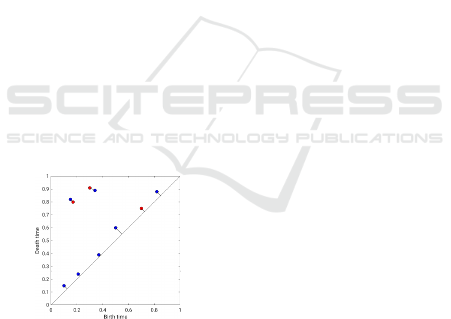
The most frequently used way to compare persis-

tence diagrams or equivalently, barcodes, with each

other is the bottleneck distance.

Deﬁnition 3.8 (Bottleneck distance). The bottleneck

distance between two persistence diagrams D

and D

is deﬁned as

∞

) = inf

ϕ:D

→D

sup

x∈D

kx − ϕ(x)k

∞

, (11)

where ϕ : D

→ D

ranges over all bijections from D

to D

. (Mileyko et al., 2011)

In words, the bottleneck distance is the longest

distance of two matched points, where the matching

between the two diagrams is chosen in an optimal

way such that it minimizes the longest distance of two

matched points. In Figure 4, one can see two persis-

tence diagrams in red and blue, respectively, and the

matching between the closest points. Points close to

the diagonal are matched to the diagonal.

In the particular case where one computes the bot-

tleneck distance of an arbitrary diagram D

and the

empty diagram D

that contains only the diagonal, all

the points in the ﬁrst diagram are matched to the di-

agonal and the bottleneck distance is proportional to

the length of the longest bar in the barcode.

Figure 4: Example for the bottleneck distance for two per-

sistence diagrams (red and blue).

4 EEG DATA

In order to apply DyCA to a multi-variate time se-

ries, a system of ordinary differential equations with

both linear and non-linear equations has to be given

to model the underlying dynamics. In (van Veen and

Liley, 2006), the authors showed via bifurcation anal-

ysis the existence of Shilnikov chaos during epileptic

seizures. The authors of (Friedrich and Uhl, 1996)

veriﬁed that the dynamics in EEG data during epilep-

tic seizures can be accurately modeled by the follow-

ing system of differential equations

˙x

= x

˙x

= x

˙x

= f (x

(12)

with f being a non-linear polynomial function.

Hence, the assumptions for applying DyCA are ful-

ﬁlled. However, if the patient is out of seizure, the

system exhibits no structure.

For the experiments, we used EEG data from a

German hospital that was measured with 25 chan-

nels using a sampling rate of 256 Hz. The data set

consists of 6 time series with lengths of 10 to 40

seconds. The EEG was recorded from patients that

suffer under a special kind of epilepsy with seizures

that are called absence seizures or petit-mal seizures.

These absences are characterized by impairment of

consciousness and an abrupt beginning and end. Usu-

ally, absence seizures last from a few seconds to half

a minute (Commission on Classiﬁcation and Termi-

nology of the International League Against Epilepsy,

1981).. We chose a moving window setup with win-

dows of 0.5 second length in order to assure that the

window size is long enough to contain at least one cy-

cle of the recurrent trajectories and short enough to

detect the absence. The beginning time of the moving

window is shifted by 0.1s, resulting in an overlap of

80% for neighboring windows.

5 NUMERICAL EXPERIMENTS

5.1 Methodology

For the preprocessing with DyCA the algorithm as de-

scribed in (Uhl et al., 2020) was used. All the compu-

tations of simplicial complexes, persistent homology

and the bottleneck distance were performed by means

of the software library JAVAPLEX (Tausz et al., 2014).

Written in Java, it can be accessed from MATLAB

and contents many relevant functions from persistent

homology. It was applied to the point-cloud data

that was obtained by applying DyCA on the entire

multi-variate time series and windowing the result-

ing four dimensional data into windows of length 0.5

seconds. This resulted in approximately 128 points

Persistent Homology based Classiﬁcation of Chaotic Multi-variate Time Series with Application to EEG Data

599

in R

per window. From this point-cloud data, a ﬁl-

tered Vietoris-Rips complex was calculated using the

JAVAPLEX library. After applying persistent homol-

ogy, the barcode for every window is calculated.

As mentioned in Section 4, during the epilep-

tic seizures one assumes that there is structure in

the data after projecting it with DyCA onto a lower-

dimensional subspace. Contrarily, in time periods

without epileptic seizures one assumes that the data

has no structure. In order to distinguish these two

states, our approach regards the 1-dimensional persis-

tent homology of the windowed, projected time-series

and compares the barcodes/persistent diagrams of ev-

ery window with the empty diagram, i.e. the diagram

which consists only of the diagonal. This is based on

the assumption that in windows without an epileptic

seizure there is no structure, hence in an ideal case

there should be no persistent features. Thus, for every

window the bottleneck distance is calculated between

the persistence diagram of the current window and the

empty diagram. For windows without an absence we

expect the bottleneck distance to the empty diagram

to be small whereas for windows where an epileptic

event is happening we expect it to be higher.

In Figure 5, one can exemplary see the results for

two windows, where Subﬁgures 5a, 5c and 5e were

generated using a window during an epileptic event

and Subﬁgures 5b, 5d and 5f correspond to a window

without an absence. The length of the windows was

chosen to be 0.7s in order to assure that the trajec-

tory shows more than two cycles. In the actual ex-

periments, a shorter window length is chosen to pre-

vent the blurring of the transition time between the

two states.

In the ﬁrst row, the trajectory projected with

DyCA is shown. To be precise, the point cloud was

projected with DyCA onto a four dimensional sub-

space, but for sake of visibility only plots in a three

dimensional subspace are shown.

In the second row, one can see the barcodes corre-

sponding to the persistent homology of both windows

in dimensions 0 and 1, respectively. The barcode dur-

ing the absence shows a completely different behavior

than the barcode in the window without an absence.

In dimension 1, one can see that there are a lot of con-

nected components during the absence until the ﬁltra-

tion value, where all connected components merge to

one component. A bit before all the connected com-

ponents except for one die, the most persistent hole

(feature in dimension 1) is born and it survives until

ﬁltration value 0.47. However, in 5c one can also see

a lot of other non-persistent holes in dimension 1, but

their lifetime is rather short. One could suspect that

the second longest bar in the barcode of dimension 1

corresponds to the little hole in the trajectory, but it is

hard to verify.

In Subﬁgures 5e and 5f, the corresponding per-

sistence diagrams for both windows are shown. Red

dots denote features in dimension 1 whereas blue dots

correspond to features in dimension 0. The triangles

denote features that do not die throughout the ﬁltra-

tion and therefore they correspond to the arrows in the

barcode of the 0-th persistent homology. As it was

already mentioned, dots that are far from the diago-

nal correspond to long bars in the barcode. Hence, in

Subﬁgure 5e the red dot that is far from the diagonal is

the persistent hole and the dots near the diagonal are

considered as topological noise. In case of the chaotic

behavior, i.e. the trajectory in the window where no

epileptic event is happening, there are no persistent

holes visible. The only holes are three holes that are

born right in the beginning of the ﬁltration and die

shortly after they are born. Hence, the multiplicity of

the red dot in the persistence diagram in 5f is three.

The barcode in dimension 0 in Subﬁgure 5d shows

that there is only one connected component through-

out the entire ﬁltration. In order to differentiate win-

dows with and without an epileptic event we consider

the most persistent hole in dimension 1 as the distinc-

tion feature.

5.2 Results

In Figure 6, the results for the bottleneck distance ob-

tained by applying the above described methodology

to the 6 different EEG time series are shown. First

of all, the given multi-variate time series is projected

onto a 4 dimensional subspace using DyCA. After-

wards, at each time step the bottleneck distance of the

persistence diagram of the point cloud in the corre-

sponding window and the empty persistence diagram

is calculated. Thus, the x-axis of every plot in Figure

6 shows the time in seconds and on the y-axis, one

can see the bottleneck distance of the window start-

ing at time x and ending at time x + 0.5s. The red

dotted lines denote the beginning and the end of an

absence, as it was detected by a medical doctor (ex-

pert). The beginning of an absence is marked with

two dotted lines at a distance of 0.5s in order to indi-

cate that the moment of the transition of the two state

can only be determined with a precision subject to the

window length. The second of the two lines that de-

note the beginning of an epileptic event is the starting

time determined by the expert.

In Subﬁgures 6a, 6b, 6c and 6f, the beginning of

the absence is detected sharply, whereas in Subﬁgures

6d and 6e the epileptic event seems to start shortly be-

fore the starting time that was detected by the expert.

ICINCO 2022 - 19th International Conference on Informatics in Control, Automation and Robotics

600

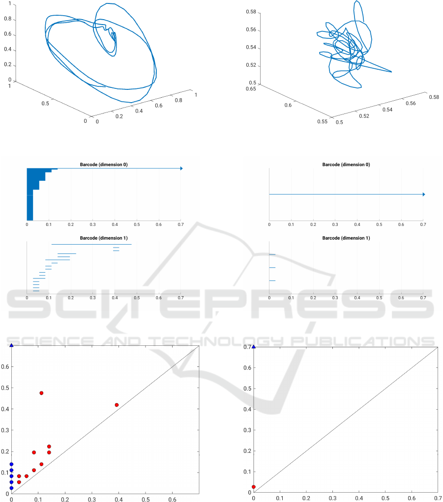
(a) Trajectory during absence.

(b) Trajectory without absence.

(e) Persistence diagram during absence.

(f) Persistence diagram without absence.

Figure 5: Overview of the results for two exemplary windows with (left column) and without (right column) an epileptic

seizure.

However, for each data set the end of an absence is

sharp and is situated exactly where it was identiﬁed

by the expert.

To get some numerical results, for every time se-

ries f

we chose a threshold α

, such that the classiﬁ-

cation task is performed in an optimal way. Windows

where the bottleneck distance is above that threshold

are classiﬁed as absence windows and windows with a

lower bottleneck distance are categorized as windows

without an epileptic event. In Table 1, one can see for

Persistent Homology based Classiﬁcation of Chaotic Multi-variate Time Series with Application to EEG Data

601

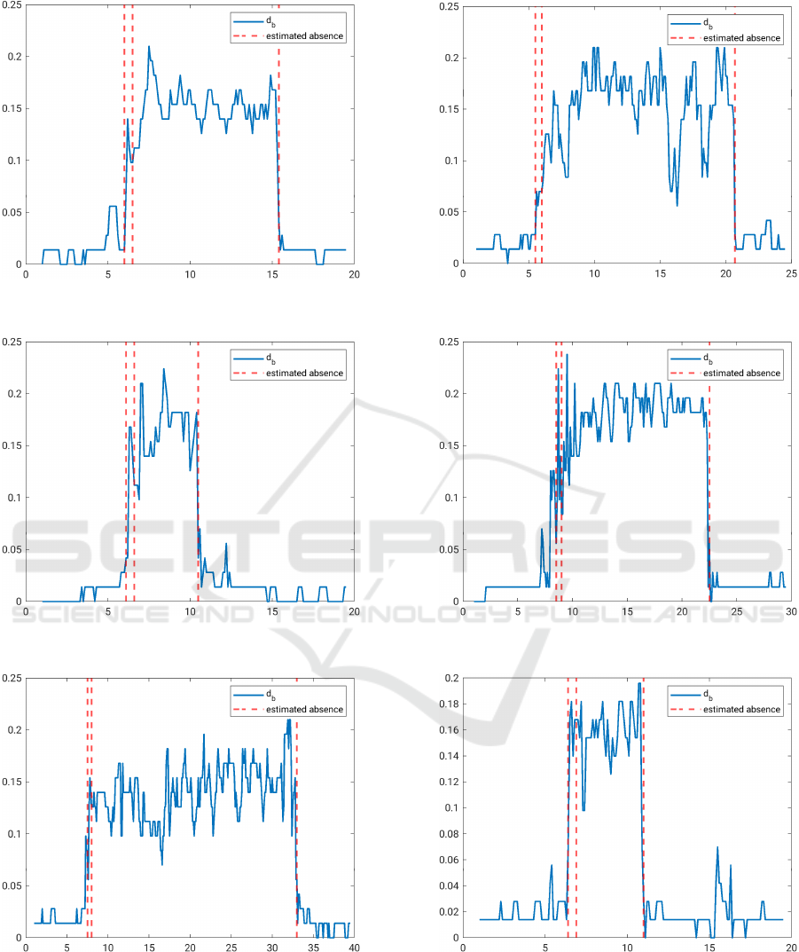
(a) Time Series 1.

(b) Time Series 2.

(e) Time Series 5. (f) Time Series 6.

Figure 6: Bottleneck distance d

for 6 data sets to detect epileptic seizures.

every time series (TS) the chosen threshold value α

and the resulting wrongly classiﬁed frames by using

the threshold. In the last column, the corresponding

percentage is shown. Since in Subﬁgures 6d and 6e

the beginning of the absence is approximately half a

second after the increase of the bottleneck distance,

it is impossible to ﬁnd a threshold α that divides the

windows into windows with or without absence.

ICINCO 2022 - 19th International Conference on Informatics in Control, Automation and Robotics

602

Table 1: Results for the classiﬁcation task of the 6 evaluated

data sets.

α Wrong frames Percentage

TS 1 0.06 0/186 0%

TS 2 0.05 0/236 0%

TS 3 0.08 1/186 0.5%

TS 4 0.08 6/286 2.1%

TS 5 0.05 4/386 1.0%

TS 6 0.08 1/186 0.5%

Even though there are some outliers, such as in

Subﬁgure 6f around second 15.6 and in Subﬁgure 6b

around second 16.3, the results show a clear differ-

ence between windows in which an epileptic event

occurs and windows without an epileptic event. Fur-

thermore, the results in Table 1 show that we achieve

a very good classiﬁcation performance with our pro-

posed approach, with the percentage of falsely cat-

egorized frames ranging from 0% to 2.1%. Addi-

tionally, it shows that without an epileptic event the

conditions of the DyCA are not fulﬁlled and hence it

fails. We conclude that the combination of DyCA and

persistent homology is well-suited to detect absence

seizures in EEG data.

6 OUTLOOK

Despite the promising results presented in the previ-

ous Section, there are still some improvements that

can be done. To be precise, EEG data can vary a lot

between different patients as well as between different

hospitals and measurement setups. Hence, the struc-

ture of the projected trajectory with DyCA can differ a

lot, making the relevant holes more or less persistent.

Also, adding a data point that lies exactly in the cen-

ter of the most persistent cycle considerably alters the

persistence diagram. Hence, even though persistent

homology is robust with respect to small perturbation

of the input data, it is not very robust with respect to

single outliers, that lie signiﬁcantly outside the struc-

ture. Future work could address this issue, either by

making the DyCA more robust or by using some so-

phisticated extensions of persistent homology.

Additionally, the structure of the attractor resem-

bles more than one loop, i.e. an outer big loop and a

smaller loop inside. However, in our investigation we

only assumed that there is one relevant hole whose

persistence was used as a classiﬁcation feature. As

an improvement, one could use more advanced tech-

niques that include the information of the entire per-

sistence diagram.

As last point, we would like to mention that the au-

thors of this paper are aware of two other papers, (Pi-

angerelli et al., 2018) and (Merelli et al., 2016), that

also investigate the use of persistent homology to de-

tect the differences between the states where epileptic

events occur (ictal states) and the states without event

or right before the event (preictal state), respectively.

To discriminate the respective states they used an en-

tropy measure that can be deﬁned on barcodes, called

the persistent entropy. By calculating a Pearson corre-

lation coefﬁcient matrix between windows of the time

series and using it as weighted edges, that give rise to

a ﬁltration of a simplicial complex, and computing

the persistent entropy of every barcode, the authors of

(Merelli et al., 2016) showed that when it comes to

the phase transition between the preictal and the ic-

tal state the number of connected components drops

to one and increases again after the phase transition.

Additionally, in (Piangerelli et al., 2018) the authors

discriminated epileptic states from non-epileptic ones

by regarding each channel as a piecewise linear func-

tion, from which a so-called lower-star ﬁltration of a

simplicial complex can be computed. From each ﬁl-

tered simplicial complex they calculated the persistent

entropy and averaged this value over all channels, us-

ing the result to train a supervised classiﬁer. They got

a strong separation of the values for the averaged per-

sistence entropy between the two states. However, the

comparison of our approach to the approaches men-

tioned above is out of the scope of this paper and will

be addressed in subsequent papers, this is ongoing re-

search.

ACKNOWLEDGEMENTS

This work has been supported by the German Federal

Ministry of Education and Research (BMBF-Projekt

05M20WWA: Verbundprojekt 05M2020 - DyCA).

REFERENCES

Commission on Classiﬁcation and Terminology of the In-

ternational League Against Epilepsy (1981). Proposal

for revised clinical and electroencephalographic clas-

siﬁcation of epileptic seizures. Epilepsia, 22(4):489–

501.

Edelsbrunner, H. and Harer, J. (2010). Computational

Topology: An Introduction. Applied Mathematics.

American Mathematical Society, Providence, RI.

Friedrich, R. and Uhl, C. (1996). Spatio-temporal analysis

of human electroencephalograms: Petit-mal epilepsy.

Physica D: Nonlinear Phenomena, 98(1):171–182.

Merelli, E., Piangerelli, M., Rucco, M., and Toller, D.

(2016). A topological approach for multivariate

time series characterization: The epileptic brain. In

Persistent Homology based Classiﬁcation of Chaotic Multi-variate Time Series with Application to EEG Data

603

Proceedings of the 9th EAI International Confer-

ence on Bio-Inspired Information and Communica-

tions Technologies (Formerly BIONETICS), BICT’15,

page 201–204, Brussels, BEL. ICST (Institute for

Computer Sciences, Social-Informatics and Telecom-

munications Engineering).

Mileyko, Y., Mukherjee, S., and Harer, J. (2011). Proba-

bility measures on the space of persistence diagrams.

Inverse Problems, 27(12):124007.

Otter, N., Porter, M. A., Tillmann, U., Grindrod, P., and

Harrington, H. A. (2017). A roadmap for the com-

putation of persistent homology. EPJ Data Science,

6(17).

Piangerelli, M., Rucco, M., Tesei, L., and Merelli, E.

(2018). Topological classiﬁer for detecting the emer-

gence of epileptic seizures. BMC Research Notes,

11(1).

Tausz, A., Vejdemo-Johansson, M., and Adams, H. (2014).

JavaPlex: A research software package for persistent

(co)homology, pages 129–136. Lecture Notes in Com-

puter Science 8592. Springer, Berlin.

Uhl, C., Kern, M., Warmuth, M., and Seifert, B. (2020).

Subspace detection and blind source separation of

multivariate signals by dynamical component analy-

sis (dyca). IEEE Open Journal of Signal Processing,

1:230–241.

van Veen, L. and Liley, D. T. J. (2006). Chaos via

Shilnikov’s saddle-node bifurcation in a theory of the

electroencephalogram. Phys. Rev. Lett., 97:208101.

ICINCO 2022 - 19th International Conference on Informatics in Control, Automation and Robotics

604