
Candle Flame Simulation Considering Temperature Change in the
Environment
Nobuhiko Mukai
1,2 a
, Reina Arai
1
and Youngha Chang
1
1
Knowledge Engineering, Tokyo City University, 1-28-1 Tamazutsumi, Setagaya, Tokyo 158-8557, Japan
2
Institute of Industrial Science, The University of Tokyo, 4-6-1 Komaba, Meguro, Tokyo, 153-8505, Japan
Keywords:
Fluid Dynamic Simulation, Particle Method, SPH, Candle Flame.
Abstract:
Fire simulations are utilized in many scenes such as explosion and conflagration in movies or games, and a lot
of techniques have been developed. Some are used to control the flame shape for animations, and others are for
real and real-time visualizations. In fact, the flame color changes according to the combustion states: complete
combustion, incomplete combustion, and non-combustion. Almost all previous studies, however, performed
flame simulations considering only one state of incomplete combustion. Then, we have been researching
the candle flame visualization considering three combustion states, and the color changed depending on the
combustion state. However, the candle flame length was too short in the previous method. Therefore, we
propose a method to consider the temperature change that affects the air density in the environment. The
change of the environmental air density induces the external force, which makes the shape of the candle flame.
As the result of the simulation, the candle flame shape has become thinner than before and has been similar to
that of a real candle flame.
1 INTRODUCTION AND
RELATED WORKS
It is said that human is the only animal who can treat
fire, and this specific character differentiates human
beings from other animals. Fire is very familiar to
us and important in our daily life. In TV dramas,
movies, and games, there are many scenes where the
fire appears such as explosions and conflagrations;
however, fire is also dangerous so careful attention
should be paid when it is treated. Then, some scenes
are generated by using computer graphics instead of
real videos; however, it is difficult to create realistic
movies by controlling the flame because the shape
changes dynamically according to the environment
such as wind, obstacles, and flammable materials.
With these backgrounds, there are many kinds
of previous research related to fire. For example,
(Louchez et al., 2006) proposed a model to simulate
and represent a candle flame by solving the Navier-
Stokes equations with a particle method, and de-
cided the shape as the NURBS (Non-Uniform Ratio-
nal B-Spline) surface that is defined with particle po-
sitions. The flame shape was physically correct; how-
a
https://orcid.org/0000-0001-8909-9454
ever, artists could not control the shape of the fire.
Then, (Bangalore and House, 2012) enabled artists to
draw fire paintings freely. Their approach was based
on the physical simulation; however, the individual
flames were drawn along the curve that artists speci-
fied by controlling the direction of the gravity and the
buoyancy. (Sato et al., 2017) also proposed a feed-
back control method for users to design a fire shape
with control points. Their method employed a PID
(Proportional Integral Derivative) controller to adjust
the force and the temperature. In addition, (Hladk
´
y,
2018) proposed a system, with which users could con-
trol the fire. Their method extended the Navier-Stokes
equations by considering the wind field, the diffusion,
the source motion, and the buoyancy terms, and the
in-between images were generated based on the hand-
drawn keyframes.
On the other hand, there are some particle-based
researches related to the simulations and the rendering
techniques of fire since it requires a lot of particles and
computational resources to simulate and visualize the
flame of fire. (Wei et al., 2002) employed the LBM
(Lattice Boltzmann Model) for physically-based sim-
ulation, and used textured splats for the rendering.
(Horvath and Geiger, 2009) also proposed a GPU-
based volume rendering method. Their method used
36
Mukai, N., Arai, R. and Chang, Y.
Candle Flame Simulation Considering Temperature Change in the Environment.
DOI: 10.5220/0011166100003274
In Proceedings of the 12th International Conference on Simulation and Modeling Methodologies, Technologies and Applications (SIMULTECH 2022), pages 36-43
ISBN: 978-989-758-578-4; ISSN: 2184-2841
Copyright
c
2022 by SCITEPRESS – Science and Technology Publications, Lda. All rights reserved
the combination of the coarse particle grid simulation,
and the fine and view-oriented refinement simulation.
In the method, the multiple independent GPUs refined
the final simulation for the rendering. In addition,
(Cha et al., 2009) used pre-calculated CFD (Com-
putational Fluid Dynamics) data to generate the fire
scene and developed a firefighter training simulator.
On the other hand, (Guay et al., 2011) proposed an
animation method to generate direct 2D images with-
out 3D simulations by considering the 2.5D velocity
field. (Sato et al., 2012) also proposed a method that
generated high-resolution 3D animations from low-
resolution fluid simulations. Their database was con-
structed with only 2D fluid simulation results, and the
low-resolution 3D simulation was performed based
on the database, and the simulation results were con-
verted to high-resolution animations.
As mentioned above, there is a lot of research on
the simulation and the visualization of fire, which
aim is to control the shape or to generate the im-
ages rapidly, and these methods are based on physi-
cal simulations. (Nguyen et al., 2002) also proposed a
method for the physically-based modeling and the an-
imation of fire. They used the incompressible Navier-
Stokes equations and considered vaporized fuels and
hot gaseous products. They also rendered the simula-
tion results with a blackbody radiation model and rep-
resented the blue core in the chemical reaction zone.
(Hamins and Bundy, 2005) simulated a candle flame
with CFD (Computational Fluid Dynamics) model
considering mass burning rate, candle regression rate,
flame height, and heat flux obtained by their experi-
ments. (Ogunedo and Okoro, 2017) also performed
CFD flow simulation on a candle flame considering
burning velocity, flame thickness, fuel flow rate, mass
consumption rate, view factor, and heat flux.
However, they did not consider the combustion
states. In fact, the flame color depends on the combus-
tion states, which are divided into three kinds: com-
plete combustion, incomplete combustion, and non-
combustion. In addition, the combustion states de-
pend on the physical property of the flammable mate-
rials. Then, (Mukai et al., 2019) proposed a method
to simulate a candle flame by estimating the physical
property of the material and to visualize the results
by discriminating the combustion states. However,
the result of the previous method showed a candle
flame whose length was too short compared to that
of a real candle. Therefore, this paper proposes a new
method to simulate and visualize a candle flame by
considering the temperature change in the environ-
ment because the temperature change affects the ex-
ternal force that elongates the candle flame.
2 CANDLE FLAME
2.1 Combustion States
Flame is divided into two types: premixed flame and
diffusion flame. Premixed flame appears when the
fuel gas and the air is uniformly premixed where the
composition of the materials, the density, and the tem-
perature are almost constant, while diffusion flame is
generated as the fuel gas diffuses being mixed with
the air when the combustion states are different and
depend on the mixture ratio of the fuel gas and the air.
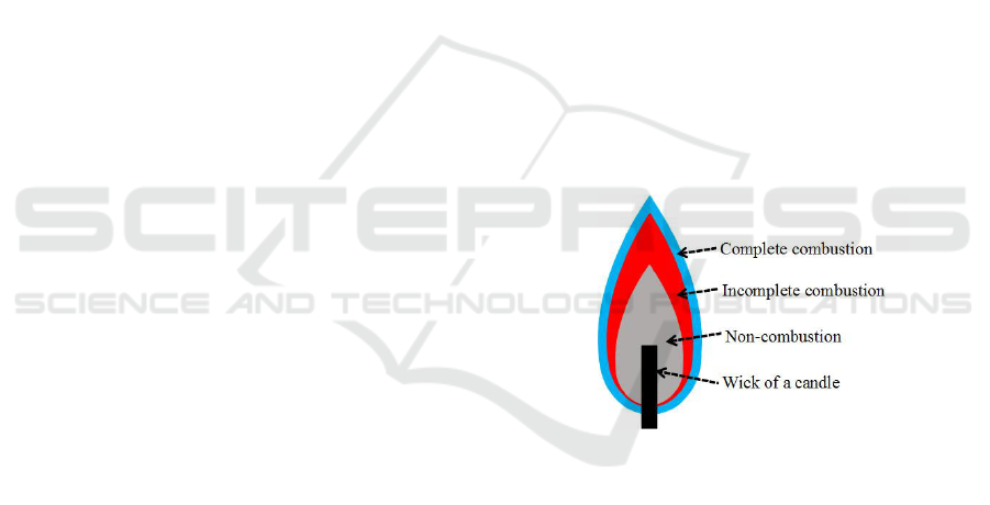
The combustion states of the diffusion flame are di-
vided into three types: complete combustion, incom-
plete combustion, and non-combustion. The color of
the premixed flame is almost constant blue although
the intensity is partly different, while the color of the
diffusion flame is different according to the combus-
tion states. The combustion states of a candle are
shown in Fig. 1. Non-combustion and the wick of the
candle are not fired so that the color is black, and the
color of the incomplete combustion is almost orange
or yellow, while the color of the complete combustion
looks blue; however, it depends on the material and is
decided by ion excitation.
Figure 1: Combustion states of a candle flame.
2.2 Candle Property
The primary component of a candle is paraffin wax,
which is the generic name of linear alkane and the
chemical formula is C
n
H
2n+2
(20 ≤ n ≤ 40); how-
ever, the composition is not clear. Then, this paper
supposes that a candle is composed of only Icosane,
which is the simplest material of linear alkanes, and
the formula is C
20
H
42
. Even if we assume that a can-
dle is composed of only Icosane, there are a lot of
unknown things that we have to estimate for the simu-
lation. The chemical formula of complete combustion
for Icosane is as follows.
2C
20
H
42
+ 61O
2
→ 40CO
2
+ 42H
2
O (1)
On the other hand, the air is composed of 78% Ni-
trogen (N
2
), 21% Oxygen (O
2
), and 1% others. Then,
Candle Flame Simulation Considering Temperature Change in the Environment
37
in Eq. (1), 61O
2
is replaced with 290Air as follows
since 290 Air includes 61(= 290 × 0.21) Oxygen.
2C
20
H
42
+ 290Air → 40CO
2
+ 42H
2
O (2)
Then, the volume ratio of complete combustion
for Icosane is 0.68 (=2/(2+290)) [vol%] since the vol-
ume ratio equals the mole ratio. This means that if the
volume ratio of the fuel gas is more than 0.68 [vol%],
the combustion state is incomplete because oxygen is
not enough for the fuel gas.
On the other hand, if the volume ratio of the fuel
gas is less than the threshold, the combustion state
becomes non-combustion since the fuel gas is not
enough. Then, the lower and the upper explosive lim-
its of the combustion state is necessary for the sim-
ulation. However, the lower and the upper explosive
limits of combustion states for Icosane are unknown.
Then, they should be estimated from the simpler ma-
terials of linear alkane, which lower and upper explo-
sive limits are shown in Table 1 (Nassimi et al., 2017).
Table 1: Lower and upper explosive limits of linear alkane.
[vol%]
Material Formula # of Lower Upper
Carbon limit limit
Methane C
1
H
4
1 5.00 15.00
Ethane C
2
H
6
2 3.00 12.40
Propane C
3
H
8
3 2.10 9.50
Butane C
4
H
10
4 1.80 8.40
Pentane C
5
H
12
5 1.40 7.80
Hexane C
6
H
14
6 1.20 7.40
Heptane C
7
H
16
7 1.05 6.70
Octane C
8
H
18
8 0.92 6.50
Nonane C
9
H
20
9 0.80 6.00
Decane C
10
H
22
10 0.70 5.00
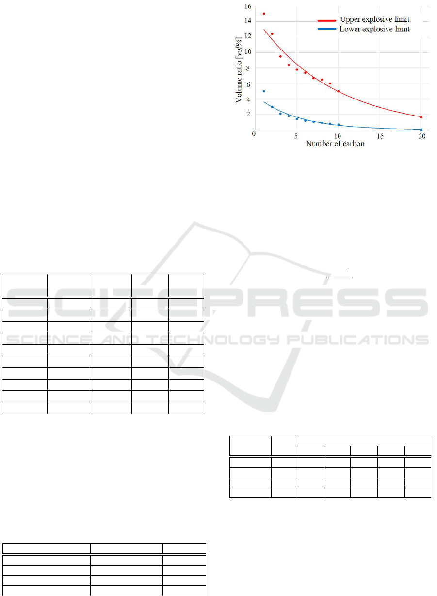
In addition, Fig. 2 shows the approximate curves
of the lower and the upper explosive limits for lin-
ear alkanes and Icosane that carbon number is 20, and
the lower and the upper explosive limits for Icosane
are estimated as 0.02 [vol%] and 1.35 [vol%], respec-
tively, from the extrapolation of the graph.
Then, the combustion states are summarized as
shown in Table 2.
Table 2: Volume ratios and combustion states of Icosane.
Volume ratio r [vol%] Combustion state Burnable
r < 0.02 non-combustion no
0.02 ≤ r < 0.68 complete yes
0.68 ≤ r < 1.35 incomplete yes
1.35 ≤ r non-combustion no
Figure 2: Approximate curves for the lower and the upper
explosive limits.
2.3 Viscosity
The viscosity of a fuel gas changes depending on the
material and the temperature. The viscosity of a mate-
rial can be calculated with Sutherland’s formula (CF-
DOnline, 2022), which is written in Eq. (3).
µ =
C
1
T
3
2
T +C
2
, (3)
where, µ is the viscosity, T is the absolute tempera-
ture, C
1
and C
2
are the constants that depend on the
material.
Then, if C
1
and C
2
are decided, the viscosity at
the specific temperature can be calculated. However,
the relationship between the viscosity and the temper-
ature of Icosane is unknown. Then, it should be esti-
mated with the simpler linear alkane, which viscosity
for the temperature is shown in Table 3.
Table 3: Viscosity of the simpler linear alkane.
[×10
−2
mPa · s]
Material # of Temperature [
◦
C]
C 0 20 50 100 200
Methane 1 1.02 1.08 1.18 1.33 1.47
Ethane 2 0.86 0.92 1.01 1.15 1.43
Propane 3 0.75 0.80 0.88 1.01 1.25
Hexane 6 0.60 0.65 0.71 0.82 1.04
Fig. 3 shows the approximate curves estimated
from Table 3, and the viscosity of Icosane, which car-
bon number is 20, can be estimated with Fig. 3.
Fig. 4 shows the relationship between the absolute
temperature and the viscosity of Icosane, which is es-
timated by plotting all points at 20 on x axis in Fig. 3.
With Fig. 4, we can estimate the viscosity from the
absolute temperature, and calculate the constants of
Sutherland’s formula, C
1
and C
2
, which are decided
SIMULTECH 2022 - 12th International Conference on Simulation and Modeling Methodologies, Technologies and Applications
38
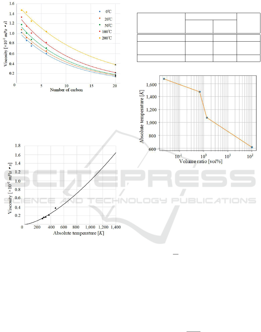
Figure 3: Approximate curves of the viscosity for simpler
linear alkanes.
as 6.95 × 10
3
and 2.21 × 10
10
, respectively. In Fig. 4,
the horizontal axis is absolute temperature [K], which
is calculated by adding 273.15 to Celsius degree [
◦
C].
Figure 4: Relationship between the absolute temperature
and the viscosity of Icosane.
The viscosity of Icosane is calculated from its
temperature with Fig. 4. On the other hand, com-
bustion states are decided by the volume ratio. Then,
the relationship between the volume ratio and the tem-
perature is necessary. Table 4 shows the relationship
between combustion states and the limit temperature
of a candle flame (ExplainThatStuff, 2022), where the
volume ratios are added according to Table 2. In addi-
tion, the boiling point of Icosane is 615.85 [K], which
volume ratio is 100 [vol%]. Then, Fig. 5 is obtained
by plotting all data, and shows the relationship be-
tween the volume ratio and the absolute temperature
based on Table 4 and the boiling point of Icosane.
Table 4: Relationship between combustion states and limit
temperatures.
Temperature Volume
Combustion State Absolute Celsius ratio
[K] [
◦
C] [vol%]
Complete (max) 1,673.15 1,400 0.02
Complete (min) 1,473.15 1,200 0.68
Incomplete (max)
Incomplete (min) 1,073.15 800 1.35
Figure 5: Relationship between volume ratio and absolute
temperature of Icosane.
3 METHOD
3.1 Governing Equations
We employ SPH (Smoothed Particle Hydrodynamics)
method for the simulation, and the governing equation
is the Navier-Stokes equations written in Eq. (4).
ρ
∂⃗u
∂t
= −∇p + η∇
2
⃗u +
⃗
f , (4)
where, ρ is the density, ⃗u is the velocity, t is the time,
p is the pressure, η is the viscosity coefficient,
⃗
f is the
external force.
Here, the density ρ(⃗x
i
) at the position of ⃗x
i
is cal-
culated as follows (Ertekin, 2015).
ρ(⃗x
i
)=
∑
j̸=i
m
j
W
d
(⃗x
j
−⃗x
i
)
=
∑
j̸=i
m
j
315
64πr
9
e
(r
2
e
− |⃗x
j
−⃗x
i
|
2
)
3
, (5)
where, m
j
is the mass of a particle j, W
d
is the kernel
function of the density, r
e
is the radius of influence,
and only ⃗x
j
within r
e
for ⃗x
i
is counted.
Candle Flame Simulation Considering Temperature Change in the Environment
39

Next, the pressure and the viscous terms at the po-
sition of ⃗x
i
are calculated as follows (Ertekin, 2015).
−∇p =−
∑
j̸=i
m
j
p
i
+ p
j
2ρ
j
∇W
p
(⃗x
j
−⃗x
i
)
=−
∑
j̸=i
m
j
p
i
+ p
j
2ρ
j
45
πr
6
e
(r
e
− |⃗x
j
−⃗x
i
|)
2
(⃗x
j
−⃗x
i
)
|⃗x
j
−⃗x
i
|
,
(6)
η∇
2
⃗u = η
∑
j̸=i
m
j
⃗u
j
−⃗u
i
ρ
j
∇
2
W
v
(⃗x
j
−⃗x
i
)
= η
∑
j̸=i
m
j
⃗u
j
−⃗u
i
ρ
j
45
πr
6
e
(r
e
− |⃗x
j
−⃗x
i
|), (7)
where, W
p
and W
v
are the kernel functions of the pres-
sure and the viscosity, respectively.
The density ρ(⃗x
i
) at the position of ⃗x
i
is calcu-
lated with Eq. (5), and suppose that the density of
the flammable material that has only the fuel gas and
no air is ρ
max
. Then, the volume ratio of a particle i,
which position is ⃗x
i
, is calculated as follows.
ρ(⃗x
i
)
ρ
max
(8)
Then, the absolute temperature of a particle is es-
timated from the volume ratio with Fig. 5, and the
viscosity (η) of the particle at the temperature is de-
rived from Fig. 4.
At last, gravity, buoyancy, and environmental air
pressure are considered as an external force. The
buoyancy works for the fuel gas and the air in the
combustion state. Then, the force that drives the
buoyancy is calculated as follows.
⃗
f
b
= (ρ
f
− ρ
e
)V
f
⃗g + (ρ
a
− ρ
e
)V
a
⃗g, (9)
where, ρ
f
, ρ
a
, V
f
, and V
a
are the densities and the
volumes of the fuel gas and the air in the combustion
state, respectively. ρ
e
is the density of the air that is
placed in the environment, which has the room tem-
perature (298.15 [K] = 25 [
◦
C]), and ⃗g is the gravity.
The environmental air pressure is calculated with
the following equation (Ueda and Fujishiro, 2014).
⃗
f
e
=−α∇p
e
=−α
∑
j̸=i
m
j
(p
e
− p
i
)
ρ
j
∇W
p
(⃗x
j
−⃗x
i
)
=−α
∑
j̸=i
m
j
(p
e
− p
i
)
ρ
j
45
πr
6
e
(r
e
− |⃗x
j
−⃗x
i
|)
2
(⃗x
j
−⃗x
i
)
|⃗x
j
−⃗x
i
|
,
(10)
p
e
= ρ
e
RT
e
, (11)
where, R and T
e
are the coefficient of the ideal gas
and the temperature of the environmental air, which is
298.15 [K] (=25 [
◦
C]), respectively, and α is the ad-
justment factor for the simulation, and 0.01 is used in
the simulation according to the experimental results.
Finally, the external force
⃗
f in Eq. (4) becomes as
follows.
⃗
f = (ρ
f
V
f
+ ρ
a
V
a
)⃗g +
⃗
f
b
+
⃗
f
e
(12)
Here, the first term of the right-hand side is the
gravity for the fuel gas and the air.
3.2 Temperature Change
In Eq. (11), p
e
can be assumed as 1.0 [atm] (= 0.1
[MPa]), and R is the coefficient of the ideal gas that
has the value (8.3145 [J/(mol · K)]). This means that
the air density in the environment (ρ
e
) can be calcu-
lated with the temperature in the environment (T
e
),
which depends on the distance from the wick of the
candle. The candle flame is vertically long, while it
is short in the horizontal direction. Then, the temper-
ature change in the vertical direction from the wick
of the candle is needed for the density calculation of
the air. However, the particles of the air in the en-
vironment are not arranged, although the particles of
the fuel gas are arranged considering the memory re-
sources and the calculation time because a lot of par-
ticles are necessary for the simulation in the particle
method. Then, the temperature of the air in the envi-
ronment must be estimated.
The temperature in the position at 10 [cm] (= 100
[mm]) in the vertical direction from the bottom of the
candle flame was measured experimentally as 298.15
[K] (= 25 [
◦
C]) that is the environmental tempera-
ture, while the temperature at the position in the hor-
izontal direction was 298.15 [K] (= 25 [
◦
C]) even if
the position was near the candle flame. Then, we
can estimate the air temperature in the vertical di-
rection with interpolation between the wick of the
candle and the position at 10 [cm] from the wick.
Here, the temperature of the wick of the candle was
1,262.44 [K] in the simulation, although the average
temperature of the incomplete state is 1.273.15 [K] (=
(1,073.15 + 1,473.15)/2[K]).
In addition, a lot of particles are needed for the
precise simulation, and in this paper, the size of the
candle is 1/4 of that in the previous research (Mukai
et al., 2019) for more precise simulation. Then,
the interpolation equation of the temperature in the
vertical direction becomes as follows.
SIMULTECH 2022 - 12th International Conference on Simulation and Modeling Methodologies, Technologies and Applications
40

T
e
[K] =
1,262.44[K] −
1,262.44[K]−298.15[K]
100[mm]/4
d
(0 ≤ d ≤ 25)
298.15[K] (Otherwise),
(13)
where, d is the distance in the vertical direction from
the wick of the candle, which unit is [mm].
4 SIMULATION AND
RENDERING
The simulation algorithm is as follows.
< Simulation Algorithm >
1. Initialization: Set parameters and place particles
around the wick of the candle.
2. Density calculation: Calculate the particle density
with Eq. (5).
3. Pressure term calculation: Calculate the pressure
term with Eq. (6).
4. Volume ratio calculation: Calculate the volume
ratio with Eq. (8).
5. Temperature decision: Decide the particle temper-
ature from the volume ratio with Fig. 5.
6. Viscosity decision: Decide the particle viscosity
at the temperature with Fig. 4.
7. Viscosity term calculation: Calculate the viscosity
term with Eq. (7).
8. Environmental temperature calculation: Estimate
the environmental air temperature with Eq. (13).
9. External force term calculation: Calculate the ex-
ternal force with Eq. (12).
10. Particle position calculation: Calculate the accel-
eration, the velocity, and the position of a particle
by solving Eq. (4).
11. Particle addition and removal: Add particles at the
wick of the candle and remove particles that have
burned out in the environment of the candle.
12. Rendering: Render the particles with the volume
rendering method, which is described in the fol-
lowing.
13. Repeat the simulation from 2.
The simulation is performed with a particle
method; however, the number of particles is not
enough for the rendering. Then, the volume render-
ing method is employed to represent a candle flame
by interpolating the density of each voxel in the grid.
The rendering algorithm is as follows.
< Rendering Algorithm >
1. Grid space decision: Set the gird space that in-
cludes all particles, and expands it from the outer-
most positions by the radius of influence.
2. Voxel size: Set the voxel size as 1.1 times the par-
ticle diameter.
3. Density set: Set each voxel density. If there are
some particles in a voxel, set the average as the
density of the voxel. If there is no particle in a
grid, set the density with IDW (Inverse Distance
Weighting) interpolation (GISGeography, 2022),
which is calculated with Eqs. (14) and (15).
The density is interpolated with the following equa-
tions.
ρ(⃗x)=
∑
N
i=1
w
i
(⃗x)ρ(⃗x
i
)
∑
N
j=1
w
j
(⃗x)
, (14)
w
i
(⃗x)=
1
d(⃗x,⃗x
i
)
p
, (15)
ρ(⃗x) is the density of the voxel at the position of ⃗x ,
d(⃗x,⃗x
i
) is the distance between the voxel at the posi-
tion of ⃗x and the particle at the position of ⃗x
i
, and p is
the order of the distance, which is 1 in this simulation.
N is the number of particles that are within the radius
of influence for the center of the voxel at the position
of ⃗x.
5 RESULTS
The simulation was performed with the PC, which
specification is shown in Table 5. The grid size for
the volume rendering changes dynamically according
to the number of particles and the space the particles
occupy. The maximum grid size was 65 × 65 × 65 =
274,625.
Table 5: Specification of the PC used for the simulation.
OS Windows 10 Education 64 bits
CPU Intel Core i5-6400
Memory 8GB
GPU NVIDIA GeForce GTX 1060
with 6 GB memory
Table 6 shows the comparison of the parameters
between the previous simulation (Mukai et al., 2019)
and the proposed one. The environmental air temper-
ature was 298.15 [K] (= 25 [
◦
C]).
The flame color in the incomplete combustion
state is decided with the linear interpolation accord-
ing to Table 7, which shows the color of the blackbody
Candle Flame Simulation Considering Temperature Change in the Environment
41
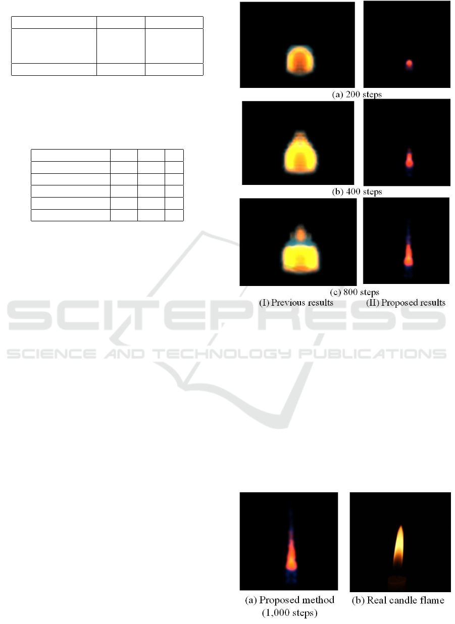
Table 6: Comparison of the simulation parameters.
Parameters Previous Proposed
Particle radius 125 [µm] 31.25 [µm]
Grid size 125 [µm] 37.50 [µm]
Time steps 800 1,000
Real time per step 1.25 [µs] 0.3125 [µs]
radiation (MitchellCharity, 2022). The temperature in
the incomplete combustion state is between 1,073.15
[K] and 1,473.15 [K] according to Table 4.
Table 7: Candle flame color.
Temperature [K] R G B
1,000 255 56 0
1,200 255 83 0
1,400 255 101 0
1,600 255 115 0
1,673 255 120 0
On the other hand, the flame color in the com-
plete combustion state is decided by ion excitation,
and there is no reference on it. Then, the color is
picked from the photograph of a real candle and de-
cided as (94, 232, 255) in (R, G, B) color space.
Fig. 6 shows the simulation results of a candle
flame. The left side images are the results in the pre-
vious simulation (Mukai et al., 2019), while the right
side images are the results in the proposed method. In
the simulation, spontaneous combustion at the wick
of the candle is supposed. In Fig. 6, the size of this
simulation is 1/4 of the previous one so the images on
the right side are smaller than those on the left side.
The shape of the flame on the right side is, however,
thinner than that on the left side and the flame is ver-
tically elongated because the proposed method calcu-
lates the external force
⃗
f
e
in Eq. (10) by considering
the temperature change in the environment with the
Eq. (13).
In addition, Fig. 7 shows the comparison of the
simulation result with a real candle flame. Fig. 7 (a)
shows the simulation results of the proposed method
at the time step of 1,000, while Fig. 7 (b) shows a
real candle flame. The shape of the flame in (a) is
similar to that in (b), and the color at the bottom of
the flame is orange in both (a) and (b); however, the
color at the tip of the flame in (a) is orange, while that
in (b) is yellow, which means the temperature in the
simulation is lower than that in the real candle. In ad-
dition, the color at the center of the flame in (a) is yel-
low, which means that the temperature of the center
is higher than that of the surroundings in the simula-
tion result (a), while the temperature of the center is
lower than that of the surroundings in the real candle.
Figure 6: Comparison of the results between the previous
and the proposed methods.
In real combustion, oxygen in the center of the candle
is less than that in the surroundings, and the state is
incomplete combustion so that the temperature in the
center is lower than that in the surroundings. On the
other hand, the surroundings of the flame have plenty
of oxygen so that the state is the complete combus-
tion, and the temperature is high although the blue
color that indicates the complete combustion is not
seen in the real candle because the color of the back-
ground is black, while the tip and the bottom of the
flame in (a) have slight blue color that indicates the
complete combustion.
Figure 7: Comparison with a real candle flame.
SIMULTECH 2022 - 12th International Conference on Simulation and Modeling Methodologies, Technologies and Applications
42

6 CONCLUSIONS
Fire is very familiar to human beings and there are
many scenes using fire in movies, games, and so on.
Then, a lot of studies have been performed to simulate
and visualize fire. Some of them are on controlling
the shape by users, and others are methods to repre-
sent realistic fire in real time. However, most previous
works treated the fire only in the incomplete combus-
tion state without the complete combustion. In addi-
tion, the most familiar fire is a candle flame; however,
the component of a candle is unknown although the
material is paraffin.
Then, we proposed a method to simulate and vi-
sualize the candle flame with a particle method by
considering the three states of combustion: com-
plete combustion, incomplete combustion, and non-
combustion in the previous method. We also assumed
that the candle is composed of only one material of
“Icosane”, and estimated the viscosity that depends
on the absolute temperature, which also depends on
the volume ratio of the fuel gas. However, the flame
shape of the simulation result in the previous method
was not similar to that of a real candle. Then, in this
paper, we have proposed a new method to simulate
the candle flame by interpolating the environmental
air temperature, which affects the density of the envi-
ronmental air that changes the external force.
As the comparison of the simulation results be-
tween the previous and the proposed methods, the
shape of the flame in the proposed method was thin-
ner than that of the previous method and was elon-
gated vertically. It was similar to the flame of the real
candle, and the overall color was also similar.
However, the color of the surroundings in the sim-
ulation result was orange, while the color of the area
in the real candle flame was yellow. In addition, the
temperature at the center of the simulated flame was
higher than that in the surroundings, while the tem-
perature at the surroundings was higher than that at
the center in the real candle flame. Then, we plan to
investigate the reasons for these differences and con-
sider the more precise simulation method in the fu-
ture.
REFERENCES
Bangalore, A. and House, D. H. (2012). A technique for art
direction of physically based fire simulation. In The
8th Annual Symposium on Computational Aesthetics
in Graphics, Visualization, and Imaging,pages 45–54.
CFDOnline (Referenced in March 2022). Sutherland’s law.
https://www.cfd-online.com/Wiki/Sutherland’s law.
Cha, M., Lee, J., Choi, B., Lee, H., and Han, S. (2009). A
data-driven visual simulation of fire phenomena. In
ACM SIGGRAPH Posters, page Article No.74.
Ertekin, B. (2015). Fluid Simulation using Smoothed Parti-
cle Hydrodynamics. Bournemouth University.
ExplainThatStuff (Referenced in March 2022). The science
of candles. https://www.explainthatstuff.com/candles.
html.
GISGeography (Referenced in March 2022).
Inverse distance weighting (IDW) in-
terpolation. https://gisgeography.com/
inverse-distance-weighting-idw-interpolation.
Guay, M., Colin, F., , and Egli, R. (2011). Screen space
animation of fire. In ACM SIGGRAPH Asia Sketches,
page Article No.10.
Hamins, A. and Bundy, M. (2005). Characterization of can-
dle flames. Journal of Fire Protection Engineering,
15:265–285.
Hladk
´
y, J. (2018). Fire simulation in 3d computer anima-
tion with turbulence dynamics including fire separa-
tion and profile modeling. International Journal of
Networking and Computing, 8(2):186–204.
Horvath, C. and Geiger, W. (2009). Directable, hight-
resolution simulation of fire on the gpu. ACM Trans-
actions on Graphics, 28(3):Article No.41.
Louchez, F. B., Leblond, M., and Rousselle, F. (2006).
Enhanced illumination of reconstructed dynamic en-
vironments using a real-time flame model. In
AFRIGRAPHAFRIGRAPH, pages 31–40.
MitchellCharity (Referenced in March 2022). What color
is a blackbody? - some pixel rgb values. http://www.
vendian.org/mncharity/dir3/blackbody.
Mukai, N., Akasaka, S., and Chang, Y. (2019). Candle
flame simulation considering combustion states. In
IIEEJ International Conferences on Image Electron-
ics and Visual Computing, page 4.
Nassimi, A. M., Jafari, M., Farrokhpour, H., and Keshavarz,
M. H. (2017). Constants of explosive limits. Chemical
Engineering Science, 173:384–389.
Nguyen, D. Q., Fedkiw, R., and Jensen, H. W. (2002). Phys-
ically based modeling and animation of fire. ACM
Transactions on Graphics
, 21(3):721–728.
Ogunedo, M. B. and Okoro, V. I. (2017). Cfd simulation
of a candle flame propagation. Elixir Journal of Me-
chanical Engineering, 108:47813–47817.
Sato, S., Mizutani, K., Dobashi, Y., Nishita, T., and Ya-
mamoto, T. (2017). Feedback control of fire simu-
lation based on computational fluid dynamics. Com-
puter Animation and Virtual Worlds, 28(3-4 e1766).
Sato, S., Morita, T., Dobashi, Y., and Yamamoto, T.
(2012). A data-driven approach for synthesizing high-
resolution animation of fire. In The Digital Production
Symposium, pages 37–42.
Ueda, K. and Fujishiro, I. (2014). Splashing liquids with
ambient gas pressure. In ACM SIGGRAPH Asia Tech-
nical Briefs, page Article No.6.
Wei, X., Li, W., Mueller, K., and Kaufman, A. (2002). Sim-
ulating fire with texture splats. In The conference on
Visualization, pages 227–235.
Candle Flame Simulation Considering Temperature Change in the Environment
43
