
Design and Validation of an Adaptive Force Control Algorithm with
Parameter Estimation Unit for Electromechanical Feed Axis
André Sewohl
1a
, Manuel Norberger
1b
, Stefan Sigg
2c
, Holger Schlegel
1
and Martin Dix
1d
,
1
Institute for Machine Tools and Production Processes, Chemnitz University of Technology, Reichenhainer Str. 70,
09126 Chemnitz, Germany
2
Fraunhofer Institute for Production Systems and Design Technology, Pascalstraße 8, 10587 Berlin, Germany
Keywords: Electromechanical Feed Axis, Force Control, Adaptive Control, Parameter Estimation.
Abstract: Production technology is characterized by the use of electromechanical feed axes, for which the concept of
cascade control has become established. The concept is based on linear control engineering. It is not suitable
for the control of process forces, which is associated with nonlinearities. Here, adaptive control algorithms
from the field of higher control engineering represent a promising approach for improvements of
manufacturing strategies and processes in terms of stability, quality, and efficiency. This can also ensure in
reducing the number of parts rejected due to bad quality and thus aiding as a significant economic benefit. In
this paper, the development of an adaptive control concept that automatically reacts to different and changing
environmental conditions during the process is presented. The digital, parameter-adaptive controller consists
of a recursive online parameter estimation unit, the controller design procedure, which is based on the setting
rule for the symmetric optimum, and the control algorithm. The functionality of the adaptive control concept
is demonstrated in simulation and validated by means of experiments on a test setup. It is real-time capable
and implemented directly on the machine control together with all calculation algorithms.
1 INTRODUCTION
Currently, production technology is subjected to the
influence of global markets more than ever and is
forced towards high productivity and economy. A
trend towards smaller batch sizes and more individual
products is currently being established without
compromising on the quality requirements, process
reliability, and life cycle costs (Tolio and Urgo,
2013). This leads to new challenges for the industry
and hence resulting in promoting the development of
flexible and adaptable machines and processes. In
modern production machines, mainly electro-
mechanical feed axes are used to generate a motion.
There are many strategies for controlling machine-
specific quantities, such as the position or speed of
electromechanical axes. The concept of cascade
structure, also known as servo control, has already
been established in this field (Leonhard, 2012).
a
https://orcid.org/0000-0003-2031-6603
b
https://orcid.org/0000-0002-0276-697X
c
https://orcid.org/0000-0002-4717-1953
d
https://orcid.org/0000-0002-2344-1656
However, the performance of this conventional
control concept at the machine level has been
exhausted. It cannot meet the ongoing efforts to
further improve the manufacturing strategies and
processes in terms of stability, quality, and efficiency.
One possibility for ensuring stable process conditions
and reducing rejected parts is closed loop control of
quality determining parameters (Allwood et al.,
2016). The development of suitable control concepts
at the process level, in which significant process
variables are taken into account as controlled values,
offers considerable scope for improvement at this
point. There are many process variables which have
an influence to the quality of a part. However, usually
it is very difficult to control these values. The
metrological acquisition of corresponding parameters
constitutes a further challenge.
The process force is a suitable parameter that can
be detected well by measurement and provides
Sewohl, A., Norberger, M., Sigg, S., Schlegel, H. and Dix, M.
Design and Validation of an Adaptive Force Control Algorithm with Parameter Estimation Unit for Electromechanical Feed Axis.
DOI: 10.5220/0011191500003271
In Proceedings of the 19th International Conference on Informatics in Control, Automation and Robotics (ICINCO 2022), pages 629-639
ISBN: 978-989-758-585-2; ISSN: 2184-2809
Copyright
c
2022 by SCITEPRESS – Science and Technology Publications, Lda. All rights reserved
629

significant economic benefits for many use cases. It
is of particular relevance for the majority of processes
in the field of production technology and often the
limiting factor for the design of the processes and the
choice of parameters. Excessive loads can cause
damage and defects to the workpiece, tool or
machine. In addition, process forces provide
important information about the process state and
allow conclusions about deviations in the production
process (Yao et al., 2013), (Allwood et al., 2016). As
a controlled variable, it is predestined to ensure
stability and safety of many processes. Direct
influence also enables increasing productivity and
improving part quality. However, there are many
challenges and requirements associated with force
control.
The process itself is part of the controlled system,
so that deviations of the controlled system and
nonlinearities occur more frequently. With classic
proportional - integral - derivative (PID) - controllers,
this results in poor performance or even instability.
PID-control forms the basis of the established cascade
control for electromechanical feed axes. The use of
higher control concepts is recommended for
controlling non-linear systems. But complex control
structures and algorithms are difficult to integrate in
machine tools with conventional industrial control.
Additional hardware usually has to be used for the
sensors and control algorithms. The resulting
communication times in turn reduce performance and
reaction speed is limited. Direct access to the control
level is necessary to ensure real-time capability. In
this context, measuring the process forces with
additional sensors is also problematic. The cycle time
is increased even further through signal processing
and integration into the control system. Due to the
delay times in signal processing, real-time capability
is not guaranteed for dynamic movements of feed
axes. High-resolution and fast measurement inputs
are particularly relevant here. Thus, the design of a
suitable control concept with real-time capability
represents a significant challenge.
In particular, adaptive algorithms that can react to
deviations of the controlled system represent a
promising approach to meet the challenges. Adaptive
control concepts have been investigated and
developed for many tasks in production engineering.
A dynamic threshold-based fuzzy adaptive control
algorithm for hard-sphere grinding processes was
introduced by (Li et al., 2012). (Vrabel et al., 2016)
examined an adaptive control system with constraints
for a drilling process. (Maher et al., 2015) developed
an adaptive neuro-fuzzy inference system, which uses
a cutting force signal for the surface roughness
prediction in computerized numerical control (CNC)
end milling. An online parameter self-adaptive force
controller for robot milling was designed in
consideration of the robot feed-direction dynamics
and the time-varying first-order model of the cutting
process by (Xiong et al., 2020). (Deng et al., 2021)
presented a learning adaptive force control concept
based on real-time object stiffness detection for
medical robots. (Calanca and Fiorini, 2018) analyzed
the behaviour of an adaptive force controller for
series elastic actuators in very different environments.
However, control of process forces in production
machines with electromechanical feed axes is still a
developing field and offers space for potential
improvement. The focus of this work is on the
development of an adaptive control concept that
automatically reacts to different and changing
environmental conditions during the process. This
ensures the stability of the control loop. In addition,
the adaptation concept with all calculation algorithms
is implemented directly on the machine control and is
real-time capable.
In the next section, the adaptation concept, its
components and functionality are explained.
Section 3 deals with the experimental set-up. The
simulation results are described in detail in section 4.
Subsequently, the execution of the experiments and
the validation of the control concept are presented in
section 5. The publication concludes with a summary
and outlook.
2 ADAPTIVE CONTROL
The application of an adaptive control concept is
suitable for preventing poor performance or
instability caused by deviations of the controlled
system or non-linearities. Non-linear adaptive
controllers have the ability to adapt the controller
parameters of the basic control loop automatically
during the process to a changing or unknown process
behaviour by means of a parameter setting unit
(Landau et al., 2011). With the independent
adjustment, an improved performance and
functionality of the controller can be achieved. A
comprehensive description on the classification and
categorisation of the different adaptive control
concepts with regard to their mode of operation and
execution principle can be found, for example, in
(Åström and Wittenmark, 2013). The structure,
components and functionality of the selected
adaptation concept are explained in the following.
ICINCO 2022 - 19th International Conference on Informatics in Control, Automation and Robotics
630
2.1 Adaptation Principle
In general, it is desirable to keep the complexity of a
controller as low as possible. In particular, real-time
capability must also be ensured for complex control
concepts. For force control, the effective stiffness in
the contact situation is the determining system
parameter. Direct measurement is not possible.
Therefore, a parameter-adaptive, indirect adaptation
is suitable for the implementation of the control
concept. Model identification adaptive control
(MIAC) is used for this purpose. Here, changes in the
controlled system are detected by an identification
stage and the control parameters are adapted on the
basis of a quality criterion. The digital, parameter-
adaptive controller typically consists of the three
methods of recursive online parameter estimation, the
controller design procedure and the control algorithm
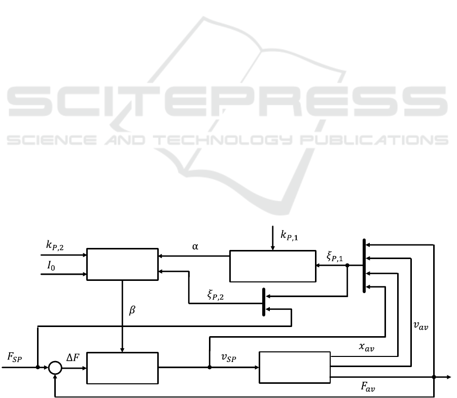
(Isermann, 1991). The basic structure is shown as a
signal flow diagram in Figure 1.
The concept is based on estimating controlled
system parameters and using this information to
calculate the basic control loop parameters. The
calculation rule for the controller parameters is called
adaptive law and results according to (Schulze and
Rehberg, 1988) to:
𝛽
𝑡
𝑓
𝐼
; 𝛼
𝑡
; 𝜉
𝑡
; 𝑘
.
(1
)
The inputs of the adaptive controller are
summarised in the form of the design criterion 𝐼
, the
constant vector 𝑘
and the signal vector 𝜉
𝑡
. The
process parameter vector 𝛼
𝑡
is calculated by
means of the estimation unit. With this, the adaptation
parameter of the basic control loop 𝛽
𝑡
is
determined in the controller design unit. Here, the
foot index 1 represents the parameters for the
parameter estimation unit and the foot index 2
represents the parameters for the controller design
unit. After selecting all free design parameters, a
parameter-adaptive controller can be put into
operation. In the start-up phase, however, an
unpredictable transient behaviour of the controller is
possible until a correct parameter estimation is
available. In this case, the adaptive controller could
be instable from the start. Therefore, a stable basic
loop controller is kept in the control algorithm as a
start model. The three essential components and
structures of the adaptive controller, including the
functionality, are explained in more detail in the
following sections.
2.2 Control Algorithm
For the control of electromechanical feed axes, the
cascade structure has established as a proven concept.
It consists of several control loops that are
superimposed on each other. In this application, the
velocity and current controller are subordinated to the
adaptive force controller. Accordingly, the control
plant of the force controller consists of the
subordinated velocity and current control loop, as
well as the mechanics of the axis and the process. This
is illustrated in the simplified signal flow diagram in
Figure 2.
The influence of the process is taken into account
by the effective stiffness K
E
. In addition, the current
control loop is shown here as a proportional-time
(PT1)-element for simplification. On the test setup,
both current and velocity controllers are implemented
as proportional-integral (PI)-controllers. Thus, the
controlled system including the process already
contains an integrating part. Therefore, the force
controller can be designed as a proportional (P)-
Figure 1: Block diagram and signal flow diagram of the parameter-adaptive controller.
Controller
Design Unit
-
Basic Control
Loop
Controlled
System
Parameter
Estimation Unit
Design and Validation of an Adaptive Force Control Algorithm with Parameter Estimation Unit for Electromechanical Feed Axis
631
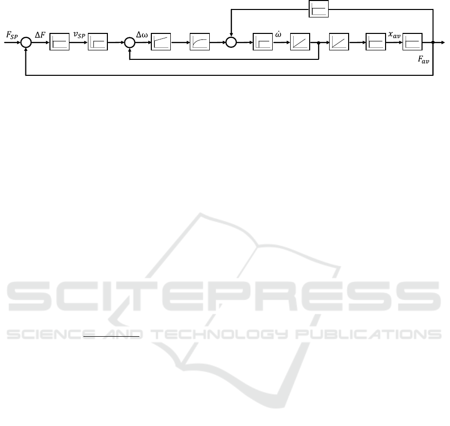
Figure 2: Simplified signal flow diagram of the basic control loop and the controlled system.
controller. This offers the additional advantage that it
can be designed quickly and easily with just one
parameter. Moreover, only one parameter then has to
be calculated and adapted during operation. This
results in less complexity, error-proneness and
calculation time, which favours real-time capability.
2.3 Controller Design Unit
The controller design is based on the setting rule for
the symmetric optimum (SO). This method is a
common design procedure for the controllers of
integrative-time (IT1)-systems. It has also proven to
be suitable in previous investigations to achieve good
performance. A more detailed description of this can
also be found in (Sewohl et al., 2020). Thus, the gain
factor K
VF
for the force controller is calculated
according to the following equation:
𝐾
1
𝑎∗ 𝐾
∗ 𝑇
.
(2)
Here 𝑎 corresponds to the damping factor, which
is usually set to the value 2. The parameter 𝑇
represents the substitute time constant of the
subordinated system. The integral gain of the force
control loop is determined by the effective stiffness
𝐾
. While the other parameters are constant, this
value varies in the process, which can lead to
instability in conventional control concepts. The
adaptive controller is aimed at making the stability
and performance of the closed-loop force control
largely independent of the stiffness 𝐾
. In order to
achieve this, the gain 𝐾
of the force controller is
adjusted in the programmable logic control (PLC)-
cycle of the control system every 2 ms. This requires
the determination of the stiffness during operation.
Direct measurement is not possible, so a parameter
estimation unit is implemented for this purpose, with
which online estimation is carried out continuously.
The estimated stiffness 𝐾
is transferred to the
controller design unit and replaces 𝐾
. In this way the
gain factor is calculated accordingly the SO.
In addition, further monitoring functions are
implemented in the controller design unit. For the
detection of a setpoint violation, a comparison of the
actual force value and the force setpoint with the
permissible difference is made. If the force control
loop starts to oscillate with a low force or
displacement amplitude, no stiffness estimation is
performed and a permanent instability may occur.
Therefore, oscillation detection is performed using a
sign comparison of the velocity setpoint from the
current and previous PLC-cycle. If one of these
criteria is violated, the parameter set for a stable basic
control loop is used. This is based on the maximum
stiffness of the controlled system. Thus, a backup
controller is kept available for critical operating
situations. After the force control loop has been
stabilised by the backup-controller, a continuous
stiffness estimation and parameter adaptation takes
place again.
2.4 Parameter Estimation Unit
Good adaptation performance requires estimation of
the effective stiffness as quickly and with as little
noise as possible. The estimation time is particularly
relevant for rapid increases in stiffness. In this case,
the force controller amplification is too high, which
results from the previous, lower stiffness. Thus, in the
event of a sudden increase in stiffness, there is a risk
of overshooting of the actual force value and even
instability of the force control loop. The low-noise
estimation is necessary because the estimated
stiffness directly influences the velocity setpoint. For
a strongly noisy parameter estimation, permanent and
distinct acceleration and braking phases would
follow. These could both reduce the lifetime of the
servo drive and negatively affect the quality of the
stiffness estimation due to dynamic inertia effects.
Thus, the task of the parameter estimation unit is to
estimate the effective stiffness online as quickly as
possible and at the same time with as little noise as
possible. This is essential for the functionality of the
adaptive controller. The basic structure is shown in
Figure 3. The parameter estimation unit consists of
M
SP
K
VF
ω
sp
T
c
K
E
-
K
P
,T
N
M
M
-
M
av
M
L
1/J
SP
ω
av
-
1
φ
AV
1
1/i
gear
i
gear
1/i
gear
ICINCO 2022 - 19th International Conference on Informatics in Control, Automation and Robotics
632
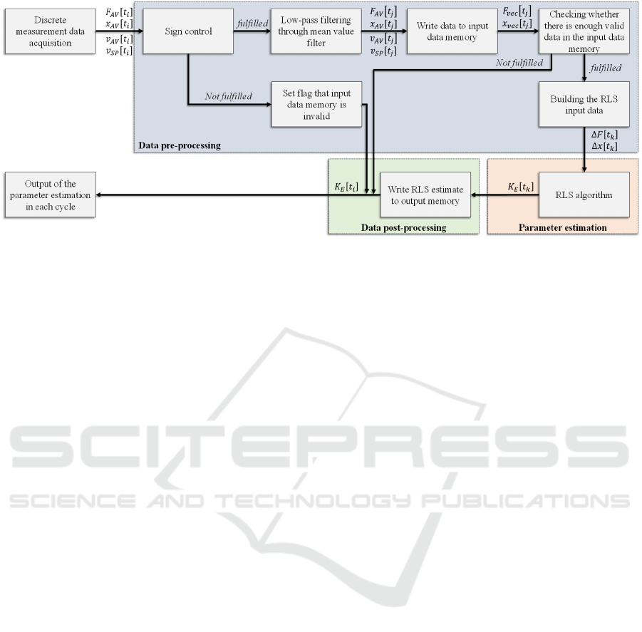
Figure 3: Basic structure and functionality of the parameter estimation unit.
the three steps of data pre-processing, parameter
estimation using the RLS-algorithm and data post-
processing. The detailed explanation of the design,
functionality and validation of the parameter
estimation unit is given in (Norberger et al., 2022).
2.5 Mode of Operation
The sequence of the PLC-program with the adaptive
force control consists of two basic sections. In the
first initialisation phase, the tool is moved at a defined
feed rate until a threshold force is reached. The
initialisation phase is necessary to obtain a reliable
estimate 𝐾
of the effective stiffness 𝐾
. An
exemplary value for the threshold force is, for
example, 50 N. When the threshold force is exceeded,
the initialisation phase ends and the adaptive force
control is activated. The adaptation cycle of the
controller runs with the following steps:
1. Initialisation: The process image as well as the
design and control parameters are imported. The
associated cycle time corresponds to the PLC
working cycle.
2. Calling the parameter estimation unit: The
stiffness is estimated from the current measured
values. The stiffness value 𝐾
is then output. If no
new stiffness estimation has taken place, the last
estimated value is used. Thus, a stiffness value is
available in each PLC-cycle. When the adaptation
unit is switched on, the initialisation estimate is
output first, which is gradually adjusted by current
estimations.
3. Calling the controller design unit: Here, the
calculation of the force controller gain 𝐾
takes
place on the basis of the SO. The information about
the force and velocity signals is also transferred to the
monitoring functions.
4. Adaptation: The controller parameter 𝐾
is
overwritten in the control loop. This parameter is used
to control the electromechanical feed axis in the
current cycle.
The controller gain is continuously adapted after
the initialisation phase according to the previously
described steps.
3 TEST SETUP
A test-setup of an electromechanical feed axis with a
control from Beckhoff was selected for the
implementation and validation of the control concept.
The basic structure of the test-setup with the
individual components is illustrated in Figure 4. The
sequence programs and operating modes, the force
control, the controller design unit with the adaptation
algorithm, the parameter estimation unit and the
setpoint generation are implemented in the IPC. This
means that all algorithms are implemented directly in
the control system. In addition, the IPC is coupled via
the backplane bus with the safety modules, I/O
modules and the measuring amplifier for the force
sensor. In this way, the communication times are
reduced from the millisecond range to the
microsecond range and the performance can be
increased. The servo inverter is connected via the
EtherCAT connection. The subordinate velocity and
current control are located here. The servo motor is
controlled here, too. In the mechanical part, the
rotational movement of the servo motor is
synchronously transmitted to the two ball screw
spindles via several belts and gears. Here exists a
mechanical forced coupling. The rotational
movement is converted into translation via the nuts
and the crosshead attached to them. In the workspace,
Design and Validation of an Adaptive Force Control Algorithm with Parameter Estimation Unit for Electromechanical Feed Axis
633
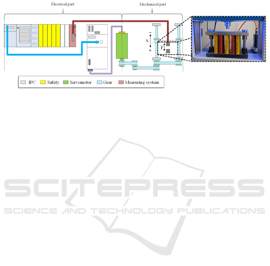
Figure 4: Experimental setup and schematic structure of the electromechanical feed axis.
the load is applied to the workpieces via the
crosshead, in which the sensor for detecting the
process forces is also integrated. The experimental
setup is designed for loads up to 10 kN. A modular
and exchangeable spring package was designed in
order to cause reproducible deviations and non-
linearities in stiffness. This load module is used to
simulate a process or a resulting process force. In this
way, variable load characteristics can be initiated
with high reproducibility by a movement of the axis
against the load module. This allows systematic
replication and investigation of changes and
deviations in the system stiffness for adaptive force
control. More detailed information on the individual
components, the commissioning and
parameterisation of the test setup can also be found in
(Sewohl et al. 2020).
4 SIMULATION
The development of the adaptive control concept was
accompanied by model-in-the-loop simulations.
MATLAB/Simulink serves as the simulation
environment. The generation of a simulation model
for the test setup has the goal of cyclically providing
the adaptive control system with a realistic process
image for iterative function tests. For this purpose, the
essential components of the adaptive control, such as
the control algorithm, the parameter estimation and
the controller design unit are created in separate
function blocks. The mechanical model of the test
setup was also inserted in a single subsystem. Due to
the modular structure, the adaptive control can be
iteratively tested and improved independently of the
test setup. Using the TwinCat C++ target for
Matlab/Simulink and the Simulink coder, it is
possible to export the control algorithm directly to the
Beckhoff machine controller.
To simulate the real system behaviour, the
mechanics of the test setup were implemented in the
simulation model as a 2-mass oscillator. The relevant
parameters, such as stiffnesses, damping, mass
moments of inertia and transmission ratios, were
determined from the technical data sheets and the
CAD-model. In addition, the signals are also
approximated as closely as possible to reality. For this
purpose, the corresponding sampling frequencies,
quantisation and noise behaviour were determined on
the experimental setup and transferred to the control
structure of the model. Computing and
communication times in the control system were also
taken into account. The implementation of a friction
model was dispensed with. The parameterisation of
the control was carried out according to the procedure
and parameters from (Sewohl et al., 2020).
Based on the comparison of real measurement
data and the response of the simulation model, a
verification of the model behaviour for relevant
operating situations was carried out. The behaviour of
the force control was examined for different
stiffnesses, force amplifications and setpoint profiles.
It was checked whether the Simulink-model can
represent the behaviour of the test setup with
sufficient accuracy for the controller design. The
contouring error as well as the starting and braking
behaviour are particularly relevant for this. The
results for a trapezoidal force setpoint profile are
shown in Figure 5. Up to the threshold value of
100 N, the feed axis is moved under velocity control.
Afterwards, the system switches to force-controlled
operation. A comparison of the contouring error as
well as the starting and braking behaviour shows that
the simulation model reproduces reality very closely.
Therefore, it is suitable for the development and
testing of the adaptive force controller. In addition to
the control structure, the controller design unit and the
parameter estimation unit were integrated into the
ICINCO 2022 - 19th International Conference on Informatics in Control, Automation and Robotics
634
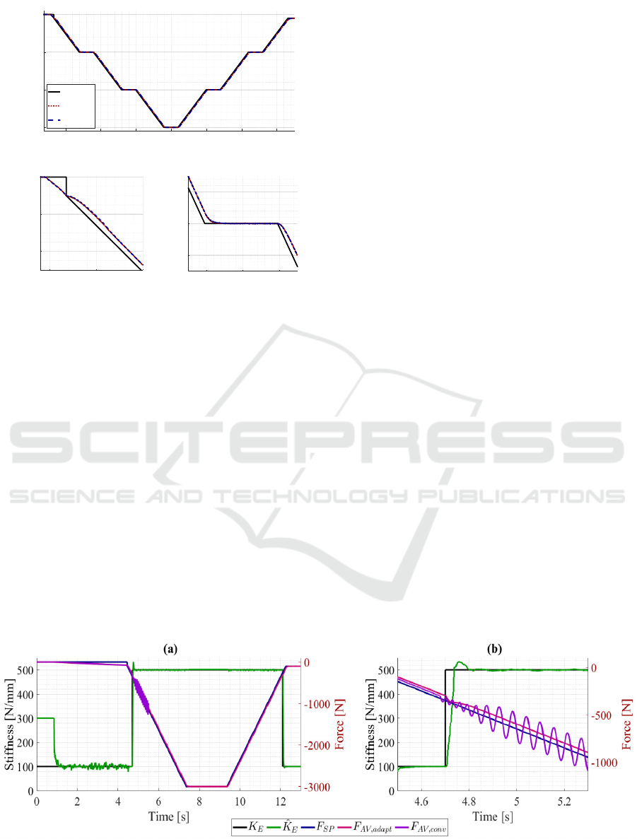
Figure 5: Comparison of actual force values from
simulation and experiment. (a) Overview of the force
profile. (b) Switching process. (c) Transition area.
model. The parameter estimation unit acts
independently of the mechanical behaviour of the test
setup and has already been validated in (Norberger et
al., 2022).
The testing of the adaptation concept in
interaction with the parameter estimation unit and the
controller design unit is first carried out in the
simulation environment using various stiffness
jumps. The reaction of the adaptive controller to a
stiffness jump from 100 N/mm to 500 N/mm is
shown in Figure 6. The diagram shows that the
adaptive controller is able to ensure a stable control
loop in the case of abrupt changes in the system
behaviour. This applies both to abrupt increases and
decreases in the effective stiffness 𝐾
. In this case,
the contouring error is also temporarily reduced or
increased. After about 50 ms, the parameter
estimation unit fully adjusts to the jump in stiffness
and the adaptive controller compensates the
contouring error again. In contrast, the conventional
controller becomes instable shortly after the change
in stiffness. For better illustration of this case, the data
are only displayed up to the time point of 5.5 s.
For the controller design, there is a freely
definable influence parameter with the design
parameter 𝐼
𝑎. This parameter is first varied in the
simulation and the results are shown in Figure 7.
Through the investigation, the effects and further
modification possibilities can be assessed. The force
curve shows that the parameter 𝑎 has an effect on the
performance. Smaller values cause smaller and higher
values correspondingly larger contouring errors.
However, small values also increase the risk of
overshooting in the event of abrupt changes and the
control loop becoming instable. But this can be
avoided by the implemented safety functions. In the
event of a setpoint violation, the parameter estimation
is stopped and the backup-controller is used. This is
illustrated in diagram (b). Diagram (c) shows the
characteristic of the controller gain 𝐾
, which is
adjusted on the basis of the stiffness estimate 𝐾
. In
the case of a setpoint violation, the calculation is re-
initiated. As soon as the parameter estimation unit
delivers reliable values again, the controller
parameter is automatically adapted.
The considered example with a sudden increase of
the stiffness from Figure 6 is to be considered as a
critical application. With a large change in the
controlled system parameters, there is a risk of an
instable control loop. It was shown that the developed
control concept nevertheless remains stable for this
critical case and the desired adaptation takes place. In
reality, such jumps are not to be expected at the test
setup. Therefore, the behaviour for a further stiffness
Figure 6: (a) Overview of the simulated behaviour of the adaptive and conventional controller during a stiffness jump. (b)
Detail of the stiffness change.
8910
Time [s]
-400
-200
0
Force [N]
(b)
12 13 14
Time [s]
-1100
-1000
-900
Force [N]
(c)
10 15 20 25 30 35 40
Time [s]
-3000
-2000
-1000
0
Force [N]
(
a
)
F
SP
F
AV
Exp
F
AV
Sim
Design and Validation of an Adaptive Force Control Algorithm with Parameter Estimation Unit for Electromechanical Feed Axis
635
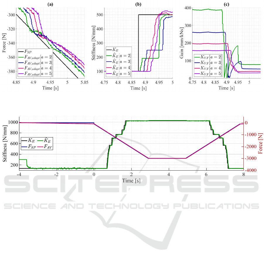
Figure 7: Influence of the design parameter a on the behaviour of the control system. (a) Comparison of the actual force
values. (b) Comparison of the stiffness estimation. (c) Comparison of the controller gain.
Figure 8: Complete profile of forces and stiffnesses for the simulative investigation of the adjusted stiffness profile.
profile is examined in the simulation. This is
approximated to the characteristic curve of the test
setup. Here, a staircase-shaped increase in stiffness
from 130 N/mm to 1000 N/mm is distributed in
several steps over the stroke process. The variation
range of the stiffness corresponds to the variation that
can actually be generated with the spring assembly.
The result is shown in Figure 8. Here it can be also
seen that the adaptive controller remains stable and
can follow the setpoint profile very well over the
entire range of variation of the stiffness change. This
is true for both compression and decompression.
Thus, the basic functionality of the concept could first
be proven in the simulation.
5 EXPERIMENTS AND
VA L I D AT I O N
In order to transfer the adaptive force control
developed in Matlab/Simulink to the test setup, it is
necessary to integrate the function modules into the
control system. Beckhoff allows direct integration of
the Simulink-model in the machine controller. For
this purpose, the model is translated into C++ code
using the Simulink code generator. The TE1400
TwinCAT Target can be used to generate a TwinCAT
Component Object model (TcCOM) from the code
(Beckhoff, 2020). The TcCOM has the inputs and
outputs defined in the Simulink model and can be
linked to a corresponding task in the Beckhoff
development environment. The inputs and outputs are
linked with the associated variables from the process
image. In this way, the two function blocks for
adaptive control with the parameter estimation unit
are transferred directly from the existing Simulink-
model to the real machine control. The algorithms are
integrated in the runtime of the machine control and
are processed cyclically in real-time.
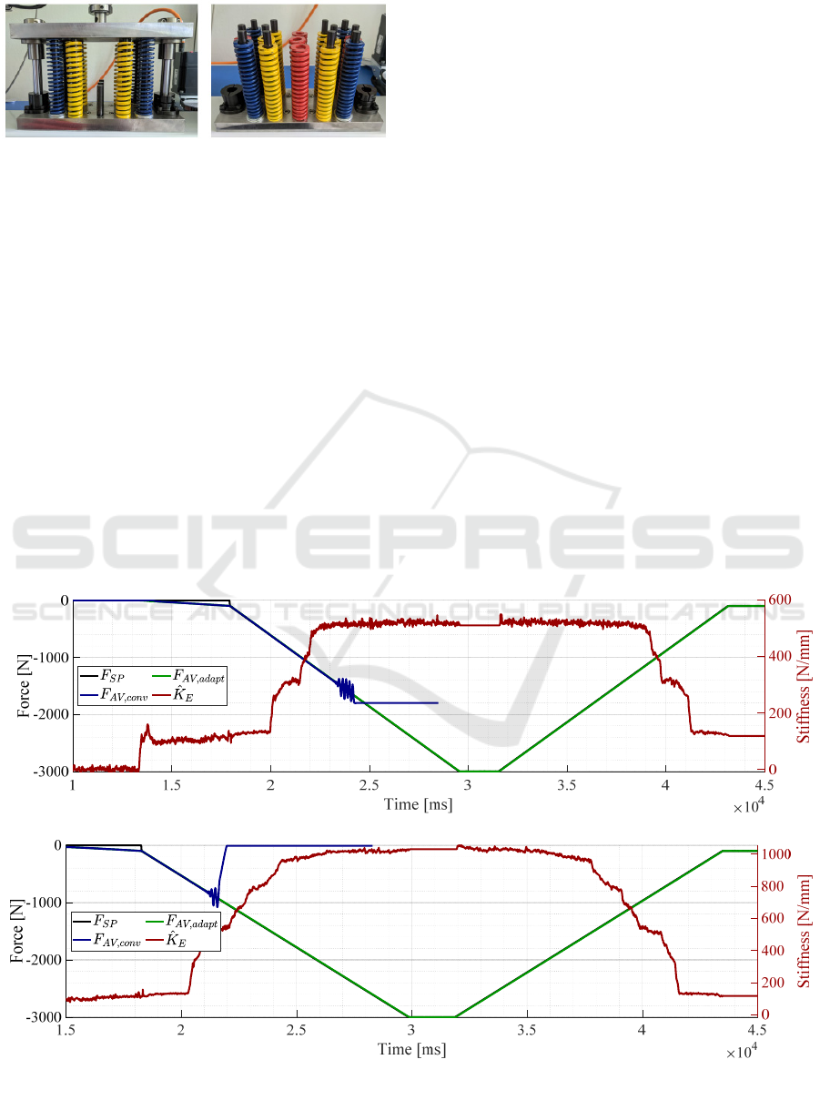
The practical testing of the concept is carried out
with the help of the modular spring package shown in
Figure 9. By combining the springs and using spacer
elements, variable path-dependent non-linear
stiffness characteristics can be specified. The
adaptive control concept is validated using the two
illustrated spring configurations with different
stiffness profiles. At the beginning of the
compression of the spring assembly, only 4 springs
are engaged. Only when the spring assembly has been
ICINCO 2022 - 19th International Conference on Informatics in Control, Automation and Robotics
636
(a) (b)
Figure 9: Combination of spring elements for stiffness
jumps. (a) Change S1 from 130 N/mm to 500 N/mm. (b)
Change S2 from 130 N/mm to 1000 N/mm.
compressed by a certain deflection do the other
springs engage. This results in a rapid increase in
stiffness. Due to the manufacturing tolerances of the
springs, there is no abrupt jump in stiffness. Rather,
the increase in stiffness from the initial to the final
stiffness takes place within a transition range of
around 2 mm. The complete curves of the
measurements for the two spring configurations are
illustrated in Figure 10. The behaviour of the
conventionally tuned force controller is also
compared here. Corresponding to the composition of
the spring assembly, the initial stiffness results in
𝐾
= 132 N/mm. The conventional controller was set
to this system behaviour without adaptation
according to the SO and the design parameter 𝑎 = 2.
During validation, the behaviour was examined at
several rates of force change (1000 N/s, 500 N/s and
250 N/s). Figure 10 (a) shows the behaviour for
250 N/s and a stiffness jump to 500 N/mm. In
Figure 10 (b) the stiffness changes to 1000 N/mm.
The stiffness changes are well reproduced by the
parameter estimation unit. It can also be clearly seen
that the conventional force controller becomes
instable and oscillates without adaptation in both
cases. Therefore, the tests were stopped at this point
by the implemented safety function and the data
recording was interrupted. The conventional force
control also became instable during all other tests. In
contrast, it is also clear that the adaptive controller
reacts very well to the change in system in practice
and follows the setpoint profile without any
instability occurring. This applies to all the tests
carried out with the three different increases in the
force setpoint ramp.
In addition, the effects resulting from a variation
of the free design parameter 𝑎 were also considered.
The results for a force increase of 1000 N/s are shown
for the stiffness jumps in Figure 11. It can be seen that
the performance of the adaptive controller can be
influenced with the free design parameter. With
smaller factors, the following error decreases, as in
the simulation. However, this also increases the
proneness to errors and the tendency to oscillate.
Figure 10: Experimental validation of the adaptive control concept. (a) Results for the stiffness jump S1. (b) Results for the
stiffness jump S2.
(a)
(b)
Design and Validation of an Adaptive Force Control Algorithm with Parameter Estimation Unit for Electromechanical Feed Axis
637
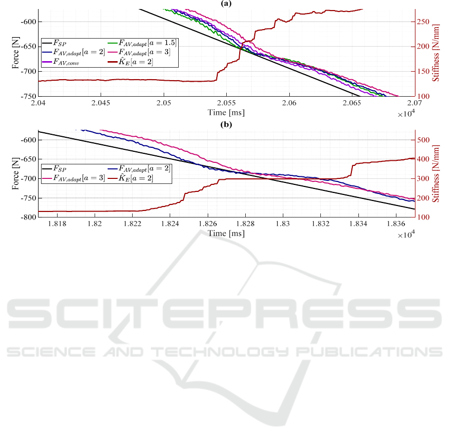
Figure 11: Measurement data of the adaptive and conventional force control for the force increase of 1000 N/s and different
design parameter 𝑎. (a) Stiffness change S1. (b) Stiffness change S2.
Conversely, larger factors result in an increased
contouring error. However, this also increases the
robustness of the control. Furthermore, the back-up
controller was implemented for the adaptive
controller as an additional safety criterion on the test
setup. This is designed for the frame rigidity of the
machine and intervenes as soon as a setpoint violation
occurs. The adaptation process is then restarted. This
functionality of the safety mechanism is illustrated in
Figure 11 (b). Here the stiffness jump S2 is shown for
a force increase of 1000 N/s. For the design factor 𝑎
= 2, a setpoint violation occurs with the change in
stiffness. In this case, the input data memory of the
parameter estimation unit is reset, the estimation is
stopped and reinitialised. This is expressed in by the
horizontal line of the parameter estimation value 𝐾
.
As soon as sufficient input data are available, new
estimated values are transferred and the adaptation
process is continued. This is the case here after about
60 ms. It can also be seen that the control then
stabilises and adjusts to the changed system. With the
use of the backup controller, the functionality of the
adaptive controller can also be ensured for critical
operating situations in practice.
6 SUMMARY
In this paper, the concept of an adaptive force
controller for an electromechanical feed axis was
presented. The individual components, the structure
and the mode of operation were explained. The
algorithm was first tested and optimised on a model
in the simulation environment. The concept was then
transferred to the test setup and experimentally
validated. In the context of this, the adaptive
controller was exported by means of the Simulink-
coder. The TcCOM was instantiated in the machine
controller and linked to the corresponding tasks,
which are processed in real-time on the PLC. The
adaptive controller behaves identically on the
machine controller to the Simulink-model in Matlab.
This principle allows optimisations and further
developments to be carried out modularly in
Matlab/Simulink and implemented with little effort.
Furthermore, it was proven in the scope of the
work that the developed controller with the parameter
estimation unit is capable of detecting changes in
stiffness and reacting to them accordingly. This
applies to both compression and decompression
processes. The adaptive controller is able to adapt the
gain factor to the controlled system during operation
based on the estimated stiffness. Even with highly
variable system behaviour, the controller remains
stable due to the adaptation of the gain factor and
improved performance is achieved. In addition, the
use of the backup-controller ensures functionality
even for critical operating situations. The behaviour
of the adaptive control can basically be influenced by
the choice of design parameters for the parameter
ICINCO 2022 - 19th International Conference on Informatics in Control, Automation and Robotics
638

estimation unit and the controller design unit.
Compared to conventional control with unchanging
parameters, an improved compromise between
stability and performance is achieved. This is
especially true if essential parameters of the
controlled system are not known a priori or are time-
variant. For small stiffness values, the adaptation
enables a higher proportional gain. At the same time,
improved stability was achieved in the range of larger
values. The investigations also demonstrated the real-
time capability of the developed control system.
Depending on the process, changes in the controlled
system are already compensated after 40-50 ms.
7 CONCLUSION AND OUTLOOK
The adaptation concept presented can be transferred
to many areas in production technology and offers a
wide range of applications. A major limitation of the
method is currently that the process force must be
dependent on the stiffness. Potential use cases are, in
particular, forming processes, material testing,
grinding, joining and assembly operations. The
concept can be used on machine tools, forming
machines and robots. Here, an analysis of the system
behaviour should first be carried out. This allows the
design parameters for the parameter estimation unit
and the controller design unit to be adjusted and
optimised to the corresponding application. In
addition, the fast responsiveness and real-time
capability are an essential characteristic of the
concept. For processes where the stiffness changes
very slowly, the design parameters and limits of the
parameter estimation algorithm have to be adapted. In
principle, it is also possible to transfer the concept to
more complex processes with different conditions. In
the case of machining operations (such as milling), it
could be used for individual force components.
Furthermore, the algorithm could also be extended or
supplemented with process models that take into
account additional influencing variables.
Future work will focus in particular on
investigating possibilities for improving the learning
phase and the switchover process for adaptive
control. In addition, an optimisation of the
empirically set design parameters is intended in
further investigations. The extension of the algorithm
with a compensation of weight and acceleration
forces is also aimed at. Furthermore, the suitability
and effects of other control structures in the control
loop shall be investigated. The safety functionalities
also still offer potential for improvement.
REFERENCES
Leonhard, W. (2012). Control of Electrical Drives - Power
Systems, Springer-Verlag. Berlin, 3
rd
edition.
Tolio, T. and Urgo, M. (2013). Design of flexible transfer
lines: a case-based reconfiguration cost assessment, In
Journal of Manufacturing Systems, 32(2), pp. 325-334.
Allwood, J. M. et al. (2016). Closed-loop control of product
properties in metal forming. In CIRP Annals –
Manufacturing Technology, 65, pp. 573-596.
Yao, X. et al. (2013). Machining force control with intelligent
compensation. In International Journal of Advanced
Manufacturing Technology, 69(5-8), pp. 1701-1715.
Li, D. et al. (2012). A dynamic threshold-based fuzzy
adaptive control algorithm for hard sphere grinding. In
International Journal of Advanced Manufacturing
Technology, 60, pp. 923-932.
Vrabel, M. et al. (2016). Monitoring and control of
manufacturing process to assist the surface workpiece
quality when drilling. In Procedia CIRP, 41, pp. 735-
739.
Maher, I. et al. (2015). Cutting force-based adaptive neuro-
fuzzy approach for accurate surface roughness prediction
in end milling operation for intelligent machining. In
International Journal of Advanced Manufacturing
Technology, 76, pp. 1459-1467.
Xiong, G. et al. (2020). Integration of optimized feedrate into
an online adaptive force controller for robot milling. In
International Journal of Advanced Manufacturing
Technology, 106, pp. 1533–1542.
Deng, Z. et al. (2021). Learning Based Adaptive Force
Control of Robotic Manipulation Based on Real-Time
Object Stiffness Detection. In arXiv preprint,
arXiv:2109.06702.
Calanca, A. and Fiorini, P. (2018). Understanding
Environment-Adaptive Force Control of Series Elastic
Actuators. In IEEE/ASME Transactions on
Mechatronics, 23(1), pp. 413-423.
Landau, I. D. et al. (2011). Adaptive control: algorithms,
analysis and applications. Springer Science & Business
Media. London, 2
nd
edition.
Åström, K. J. and Wittenmark, B. (2013). Adaptive control.
Dover Publications. Mineola, 2
nd
edition.
Schulze, K.P. and Rehberg, K.-J. (1988). Design of Adaptive
Systems - A Presentation for Engineers. Verlag Technik,
Berlin. (in German)
Isermann, R. (1991). Digital Control Systems - Volume 2:
Stochastic Control, Multivariable Control, Adaptive
Control, Applications. Springer, Berlin.
Sewohl, A. et al. (2020). Performance Analysis of the Force
Control for an electromechanical Feed Axis with
Industrial Motion Control. In ICINCO2020, pp. 667-674.
Norberger, M. et al. (2022). Development and Validation of
a Model for Online Estimation of Process Parameters for
Adaptive Force Control Algorithms. In Proceedings of
the 2
nd
Winter IFSA Conference ARCI2022, (ed. Yurish,
S.Y.), 006, pp. 19-24.
Beckhoff Automation GmbH, (2020). Manual - TC3 Target
for Matlab/Simulink, TwinCAT 3, TE1400. Beckhoff
Automation GmbH.
Design and Validation of an Adaptive Force Control Algorithm with Parameter Estimation Unit for Electromechanical Feed Axis
639
