
Efficient IoT Device Fingerprinting Approach using Machine Learning
Richmond Osei
1
, Habib Louafi
2
, Malek Mouhoub
1 a
and Zhongwen Zhu
3
1
Department of Computer Science, University of Regina, Regina, SK, Canada
2
Department of Computer Science, New York Institute of Technology (Vancouver Campus), Canada
3
GAIA Montreal, Ericsson Canada, Montreal, Canada
fi
Keywords:
Internet of Things IoT, Device Fingerprinting, Feature Extraction, Dimensionality Reduction, Machine
Learning.
Abstract:
Internet of Things (IoT) usage is steadily becoming a way of life. IoT devices can be found in smart homes,
factories, farming, etc. However, skyrocketing of IoT devices comes along with many security concerns
due to their small and constrained build-up. For instance, a comprised IoT device in a network presents a
vulnerability that can be exploited to attack the entire network. Since IoT devices are usually scattered over
vast areas, Mobile Network Operators resort to analyzing the traffic generated by these devices to detect the
identity (fingerprint) and nature of these devices (legitimate, faulty, or malicious). We propose an efficient
solution to fingerprint IoT devices using known classifiers, alongside dimensionality reduction techniques,
such as PCA and Autoencoder. The latter techniques extract the most relevant features required for accurate
fingerprinting while reducing the amount of IoT data to process. To assess the performance of our proposed
approach, we conducted several experiments on a real-world dataset from an IoT network. The results show
that the Autoencoder for dimensionality reduction with a Decision Tree Algorithm reduces the number of
features from 14 to 5 while keeping the prediction of the IoT devices fingerprints very high (97%).
1 INTRODUCTION
Internet of Things (IoT), known as the Internet of
Object usage, is gradually becoming a way of life.
IoT combines a network of physical components (sen-
sors, cars, and other items) that interact with each
other and other computing components to achieve
specific goals. Various IoT devices are continuously
introduced to cyberspace. IoT devices can be found
in many places, including transportation, healthcare,
smart homes, and even industrial environments. It has
been predicted, in (AB, 2015), that by 2022, about
29 billion devices (including 18 billion IoT devices)
will be connected to cyberspace, which will raise se-
rious security concerns. Because of IoT limited re-
sources and complexity in built-up infrastructures, at-
tackers are primarily interested in hacking IoT de-
vice networks. Attacks targeting IoT devices tend to
make IoT devices not function as expected, creating
an anomaly in the entire network. Devices showing
abnormal behavior can be detected by analyzing the
traffic they generate.
After the MIRAI botnet attack (Antonakakis et al.,
a
https://orcid.org/0000-0001-7381-1064
2017), protecting IoT devices became very promi-
nent, shutting down several big companies’ servers.
This attack exploited the weakness of millions of IoT
devices and used them to perform Distributed Denial
of Service (DDoS) attacks on DNS servers of several
big companies, such as Twitter. Because of the mas-
sive and diverse number of IoT device models, rely-
ing on the most typical approaches of device detec-
tion is becoming increasingly difficult. In this regard,
device fingerprinting offers a more efficient and effec-
tive way to collect data on devices that will aid in their
detection and help to identify security vulnerabilities
reliably (Antonakakis et al., 2017).
Device fingerprinting is the process of identifying
the identity of an IoT device from its traffic. The fin-
gerprints and their behavior baseline help drastically
detect potential attacks on IoT devices (Bratus et al.,
2008).
In this context, we present a new approach, based
on supervised machine learning (ML), capable of ac-
curately fingerprinting IoT devices connected to a net-
work. The proposed approach will first use ML di-
mensionality reduction techniques (such as PCA and
Auto-Encoder) to extract the most relevant features
from the original dataset. A classifier will then be per-
Osei, R., Louafi, H., Mouhoub, M. and Zhu, Z.
Efficient IoT Device Fingerprinting Approach using Machine Learning.
DOI: 10.5220/0011260500003283
In Proceedings of the 19th International Conference on Security and Cryptography (SECRYPT 2022), pages 525-533
ISBN: 978-989-758-590-6; ISSN: 2184-7711
Copyright
c
2022 by SCITEPRESS – Science and Technology Publications, Lda. All rights reserved
525

formed on the extracted features to perform the pre-
diction phase. To assess the performance of our pro-
posed approach, we conducted several experiments
on a real-world dataset from an IoT network. Sev-
eral known classifiers and dimensionality reduction
techniques are considered in this regard. The re-
sults obtained and reported in this paper show that the
Autoencoder for dimensionality reduction combined
with a Decision Tree Algorithm reduces the number
of features from 14 to 5 only while keeping the predic-
tion of the IoT devices fingerprints very high (97%)
2 RELATED WORK
This section reviews the most important approaches,
solutions, and frameworks proposed to fingerprint IoT
devices using ML algorithms. The literature review
will be organized into two main subsections: solu-
tions related to fingerprinting IoT devices and dimen-
sionality reduction techniques applied in ML.
2.1 IoT Device Fingerprinting
(Thangavelu et al., 2018) proposed a methodology
called a Distributed IoT Fingerprinting Technique
(DEFT), an approach for fingerprinting IoT devices
by considering the traffic session. The authors ignore
the packet level, especially the application protocol
layer (packet size, sender’s IP, and port number), even
though it is noticeably the best feature due to its cost.
The authors considered features from protocols like
DNS, mDNS, TLS., HTTP, etc. Later, Principal Com-
ponent Analysis (PCA) analyzes the features with two
components, the related 2-D planes, without reducing
the number of dimensions of the features. ML algo-
rithms were used, such as Random Forest, K-NN, and
Naive Bayes. The higher accuracy was obtained with
Random Forest. The precision reference, recall ref-
erence, and F-1 score reference metrics were used to
evaluate the accuracy of the obtained fingerprints of
the IoT devices.
In (Acar et al., 2020), the authors first proposed
a new multi-stage privacy attack on IoT devices to
leak sensitive user information. The authors evaluated
the proposed attack using the known commercial IoT
home devices dataset. Finally, they presented a solu-
tion based on traffic spoofing to effectively address
the proposed attack. Using features such as mean
packet length, mean inter-arrival time, and standard
deviation in packet lengths, the authors adopted ma-
chine learning algorithms including KNN, XGBoost,
Decision Tree, Ada Boost, Random Forest and Na
¨
ıve
Bayes. The proposed solution achieves an accuracy
of 94% with Random Forest.
(Zhang et al., 2021) propose an approach to fin-
gerprint IoT devices using an unsupervised learn-
ing framework. Unsupervised learning was chosen
over regular supervised learning due to labeling costs.
These costs correspond to the time needed to label
the dataset and human error. The authors selected
14 temporal and spatial main features to form a 72-
dimensional vector reflecting the physical attributes
of various IoT devices at the network level. Using
Variational Autoencoder to build a clustering frame-
work and K-means algorithm, the proposed method
achieved an accuracy of 86% for a given dataset.
In (Msadek et al., 2019), Nizar et al. used features
from the application protocol, transport, network, and
data link layers to develop a model to fingerprint IoT
devices. The authors offered a method to fingerprint
IoT devices by performing various evaluation and
exploration measurements on the dataset using ma-
chine learning algorithms. The proposed methodol-
ogy yielded an accuracy of 18.5% and clocked a speed
of 18.39 faster than the usual baseline approaches.
2.2 Dimensionality Reduction
In (Sakurada and Yairi, 2014), Sakurada et al. pro-
posed a method of detecting anomalies in telemetry
data of a spacecraft, using dimensionality reduction
techniques. The authors used Autoencoder to per-
form dimensionality reduction, as most of the vari-
ables in the telemetry data are not correlated. They
applied Autoencoders on synthetic and real data, and
compared the performance of Autoencoders to PCA.
It was reported that the Autoencoder detects anoma-
lies where linear PCA failed. Overall, the Autoen-
coders increase accuracy through denoising (i.e., by
randomly changing some corrupted values of the in-
put values to zero).
In (Abdulhammed et al., 2019), the authors pro-
posed a network intrusion detection system based
on ML algorithms. They used the dataset from CI-
CIDS2017 (Yulianto et al., 2019). In building the
proposed system, Autoencoder and PCA were used
for dimensionality reduction to compress and trans-
form features into a lower dimension of all the fused
data. Using these dimensionality reduction tech-
niques, the authors reduced the dataset features from
81 to 10. They maintained an overall accuracy of
99.6 % in the training process using Random For-
est, Bayesian Network, Linear Discriminant Analysis,
and Quadratic Discriminant Analysis.
Table 1 summarizes the reviewed solutions re-
ported in this section, along with their advantages and
drawbacks.
SECRYPT 2022 - 19th International Conference on Security and Cryptography
526

Table 1: Related Work Summary.
Solutions Features Strengths Weaknesses
DEFT (Thangavelu
et al., 2018)
• DNS
• mDNS
• Session statistics
• TLS
• HTTP
• SDDP
• QUIC
• MQTT
• STUN
• NTP
• BOTTP
• Use of protocols fea-
tures, which are con-
sidered less expensive
than application layer
features.
• DEFT approach can
be used to distinguish
anomalous behaviours
since it can characterize
the normal process of an
IoT device by its vendor.
• Use of protocol features instead of
the best features (application layers
features)
• It uses many features that corre-
spond to more time and resources in
the machine learning process.
• Another issue of the DEFT solu-
tion is that its scope is restricted
to local IoT networks. Thus, it
does not present an Internet-wide
view and does not apply to one-
way scan flows incoming at network
telescopes.
Peek-a-
Boo (Acar
et al., 2020)
• Mean packet length
• Standard deviation in
packet lengths
• Mean inter-arrival time
• Ability to fingerprint IoT
device is real-world ap-
plication
• The system yet effective
mitigation mechanism to
hide the actual activities
of the users from the out-
side world.
• This model raises critical privacy
concerns for any IoT devices, espe-
cially personal homes, residences,
offices of corporations or govern-
ment agencies.
Unsupervised
IoT Finger-
printing
Method
via Varia-
tional Auto-
encoder
and K-
means (Zhang
et al., 2021)
• Temporal Features (Peri-
odicity and Burstiness),
• Spatial Features (Volume
statistics features, Two-
tuple Bag features, Pro-
tocol features, Payload
features)
• Use unsupervised learn-
ing approach rather than
supervise to save the cost
of labelling and human-
error in labelling
• The accuracy of this model is low
compare with other IoT fingerprint-
ing models.
• Because this algorithm uses an un-
supervised learning process, It will
take a lot of time to calculate and an-
alyze data.
IoT Device
Fingerprint-
ing: Machine
Learning
based En-
crypted
Traffic Anal-
ysis (Ab-
dulhammed
et al., 2019)
• Application layer
(HTTP, HTTPS, DHCP,
SSDP, DNS, MDNS,
NTP, SMB, AFP, SSH)
• Transport layer (TCP,
UDP)
• Network layer (IP, ICMP,
ICMPV6, IGMP)
• Data link layer(ARP,
LLC)
• The proposed methodol-
ogy yielded an accuracy
of 18.5% and clocked
a speed of 18.39 faster
than the usual baseline
approaches.
• The model depends on handcrafted
parameter tuning and does not seg-
ment traffic autonomously as we do
in this work.
• The proposed solution works only
for massive training datasets con-
taining no noise.
• The solution is not a stand-alone
system but instead, rely on other ap-
proaches to fingerprint and provide
proper security.
Efficient IoT Device Fingerprinting Approach using Machine Learning
527
3 PROBLEM STATEMENT
It is assumed that we have an IoT network to which
a set of IoT devices are attached. Our objective is to
analyze the traffic generated by these IoT devices and
identify (fingerprint) their identities (e.g., the device’s
name). It is known that the network traffic of IoT de-
vices is huge. Thus we are more interested in identify-
ing the minimal set of features needed to fingerprint
the IoT devices, with the highest accuracy possible.
To that goal, we experiment with various dimension-
ality reduction techniques, such as PCA and Autoen-
coders, to find the optimal set of features capable of
fingerprinting IoT devices. The problem at hand can
be formulated as follows.
Let R be a set of known dimensionality reduc-
tion methods, and F the set of all the features that are
initially extracted (in the sense of ML) from a given
dataset D. Let us denote each combination of fea-
tures by f
i
. f
i
⊆ P(F) where P(F) represents the
power of the set F (1 ≤ i ≤ 2
|F|
. As stated earlier,
our methodology combines a given dimensionality re-
duction method, r
j
, with a classifier m
k
. Our ulti-
mate goal is to find the optimal combination (r
∗
, m
∗
)
minimizing the prediction score, measured using one
known prediction metric (accuracy, precision, recall,
or F1-Score). This problem can be formulated using
Equation 1.
(r
∗
, m
∗
) = argmax
r
i
∈R ,m
i
∈M
S
p
(r
i
, m
i
) (1)
where, R and M are respectively, the set of dimen-
sionality reduction techniques and the set of classi-
fiers. r
∗
returns the optimal set of extracted features
f
∗
.
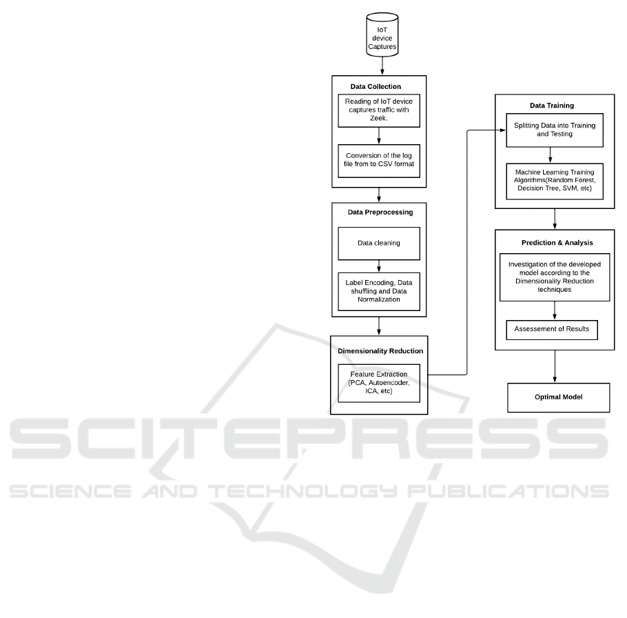
4 METHODOLOGY
To solve equation (1) and find the optimal subset of
features that can be used to fingerprint the IoT de-
vices, while keeping the prediction score higher, we
propose a system comprised of several modules, as
shown in Figure 1. In the following, these modules
are described.
4.1 Data Collection
The data preparation phase includes acquiring the IoT
device data captured and converting it into a readable
ML format for data preprocessing. The IoT device
captures are recorded in pcap files, which we pro-
cessed using Zeek (formerly Bro) and obtained differ-
ent log files. Some of the Zeek obtained logs include
Figure 1: Proposed methodology flowchart.
conn. log, dhcp.log, dns.log, ntp.log, ssh.log, ssl.log,
Z509.log. Here we are more interested in the con-
nection logs, as they contain the most important in-
formation about the traffic (Gustavsson, 2019). Then,
the connection logs are converted into CSV files, to
which we add the labels, which are the names of the
devices.
4.2 Data Preprocessing
Data preprocessing refers to the process of data clean-
ing, label encoding, data shuffling, and data normal-
ization. This process is crucial for the ML algorithm
to be able to efficiently process datasets, which in
turn increases the accuracy of the ML performance.
It eliminates defective elements (e.g., missing data,
duplicate instances) and outliers (Garc
´
ıa et al., 2015).
In natural world settings, it is impractical to ob-
tain a flawless dataset due to errors in data ac-
quisition/collection, device limitation, or human er-
rors (Van den Broeck et al., 2005). Therefore, in
the data cleaning process, we remove some data from
the dataset that does not conform to the pattern or is
considered unnecessary. The following steps are con-
ducted to cleanse the dataset under consideration:
• Deletion of rows with missing or duplicate values.
SECRYPT 2022 - 19th International Conference on Security and Cryptography
528

• removal of inconsistent values according to the
feature data type. i.e. that instances that do not
fit features.
• and removal of columns that have low variance.
The MinMaxscaler is used to normalize the
dataset by shifting and scaling the values in a range
of 0 and 1.
X
scaled
=
x − min(x)
max(x) − min(x)
(2)
where, min(x) amd max(x) are respectively the mini-
mum and maximum values of the feature x.
4.3 Dimensionality Reduction
First, feature selection techniques are applied to dis-
card the non-relevant features and keep only those
that are really needed. Then, feature extraction tech-
niques are perfomed to extract the most relevant com-
ponents. Feature extraction improves prediction ac-
curacy and computational efficiency by reducing data
redundancy (instances having a linear correlation with
each other (Wang et al., 2016). We consider the fol-
lowing linear or non-linear dimensionality reduction
techniques.
• Linear Dimensionality Reduction Techniques:
– Principal Component Analysis (PCA): PCA
is selected in this research based on its lin-
ear transformation technique to check for lin-
earity between various features in the dataset
(Anowar et al., 2021).
– Independent Component Analysis (ICA): ICA
too was selected based on its linear and super-
vised transformation technique but unlike PCA.
ICA was used to search for a linear direction of
non-Gaussian data, and the components are in-
dependent statistically (Comon, 1994).
– Linear Discriminant Analysis (LDA): LDA se-
lection too was based on its linearity and it’s
being a supervised dimensionality technique.
(Anowar et al., 2021). Similar to PCA, but
apart from maximizing the data variance, it also
maximizes the separation of multiple classes.
(Reddy et al., 2020). Minimum components of
5 resulted in the highest accuracy
– Exploratory Factor Analysis (FA): Factor Anal-
ysis was chosen also because of the linear
transformation technique. Unlike PCA, EFA
only considers common variance, while PCA
considers both specific and common variance.
(Schreiber, 2021). Minimum components of 4
resulted in the highest accuracy.
– Non-Negative Matrix Factorization (NMF):
Non-negative Matrix Factorization was cho-
sen also because of the linear transformation
technique. In contrast with PCA and ICA,
NMF made non-negativity constraints making
the representation only additive (allowing no
subtractions), in contrast to many other linear
illustrations such as PCA and ICA. (Cai et al.,
2008).
– Karhunen Loeve Transform (KLT): Karhunen-
Loeve Transform (KLT) was selected based on
the linear dimensionality reduction technique.
Closely related to PCA, but unlike PCA it looks
for the reversible transformation by eliminat-
ing redundancy by removing a dataset’s corre-
lation (Rao and Yip, 2018). Minimum compo-
nents of 5 resulted in the highest accuracy
• Non- Linear Dimensionality Reduction
Tecnhinques
– SparsePCA: Like PCA, Sparse PCA was cho-
sen because of its non-linear dimensionality
technique to check for non-linearity between
some features in the dataset. Compared to
PCA, in Sparse PCA, the principal components
are selected as components with fewer non-zero
values in their coefficient vectors. Also, Sparse
PCA does not solve data interpretation issues
concerned with PCA but solves the inconsis-
tency of the calculating component weights
in the high-dimensional setting (Guerra-Urzola
et al., 2021).
– Autoencoder (Autoencoder): Autoencoder was
chosen basically because of its local non-linear
reduction technique. That produces a better
performance on manifolds where the “local ge-
ometry is close to Euclidean” (Silva and Tenen-
baum, 2002)., but the “global geometry is prob-
ably not”. In this research, the Autoencoder
ANN was used using the TensorFlow autoen-
coder library in python.
4.4 Data Training and Prediction
Analysis
Different supervised ML algorithms are applied to the
dimensionality-reduced dataset in training the model.
Hyper-parameter tuning was adopted in the classifica-
tion algorithms used, for example, choosing the best
K value for KNN, the maximum depth for the deci-
sion tree algorithm, the number of trees for the ran-
dom forest classifier, and the number of layers used
in generating a bottleneck for Autoencoder. Using
the SKlearn library in Python, extracted components
Efficient IoT Device Fingerprinting Approach using Machine Learning
529

from the dimensionality algorithms were partitioned
80/20 percent for training and testing.
In order to prevent the effect of unbalancing data
in regard to each class label, a stratified train/test split
(a default in SKLearn library) is adopted. The ac-
curacy (precision, recall and F1-score) average of 10
was taken for each machine learning algorithm. These
algorithms are as follows: Random Forest (RF), Deci-
sion Tree (DT), K-Nearest Neighbors (KNN), Naive
Bayes (NBC), Super Vector Machine (SVM).
4.5 Prediction and Analysis
The trained models obtained for each ML algorithm
and feature extraction method listed earlier are com-
pared to identify the optimal ones that solve (1). That
is, the feature extraction method and ML algorithm,
which yield the least number of features and highest
accuracy simultaneously, are selected as the optimal
ones. The performance used metrics are as follows:
Precision, Recall, and F1-Score.
5 EXPERIMENTATION
5.1 Experimentation Environment and
Dataset
We have used a Dell computer with an 11th Gen In-
tel(R) Core(TM) i9-11900K @ 3.50GHz, a Random
Access Memory(RAM) of 64GB, and a Graphics
Processing Unit(GPU) of 6GB (Nvidia GTX 1660
Ti). We are using Zeek, a passive, open-source
Unix-based network traffic analyzer, to monitor the
traffic from the dataset (Miettinen et al., 2017). An
MS- Excel to clean and label the dataset. The process
is run using Juptyer Notebook 6.3.0 on Anaconda
2.1.0 (Perez and Granger, 2015), with libraries,
including Pandas, NumPy, SKLearn, Matplotlib, and
Tensorflow (Pedregosa et al., 2011).
The dataset used in the ML process is real-world
data that is captured from a real IoT network (Miet-
tinen et al., 2017). The latter comprises 31 IoT de-
vices, from which 27 devices are of different types
(meaning that four types are represented by two de-
vices each). The different device types are presented
in Table 2, and the set of features is listed in Table 3.
From this list of 17 features, only 14 are kept after
performing feature selection (Time, UID, and History
are removed). The schema of the dataset, including
the number of instances, is shown in Table 4. We
consider all the four classification methods listed in
Table 2: IoT device types (Miettinen et al., 2017).
No. Device No. Device
1 Aria 15 HomeMaticPlug
2 D-LinkCam 16 HueBridge
3 D-LinkDayCam 17 HueSwitch
4 D-LinkHomeHub 18 iKettle
5 D-LinkSenor 19 Lightify
6 D-LinkSiren 20 MAXGateway
7 D-LinkSwitch 21 SmarterCoffee
8 D-LinkWaterSensor 22 TP-LinkPlugHS100
9 EdimaxCam 23 TP-LinkPlugHS110
10 EdimaxPlug1101W 24 WeMoInsightSwitch
11 EdimaxPlug2101W 25 WeMoLink
12 EdnetCam 26 WeMoSwitch
13 EdnetGateway 27 Withings
14 D-LinkDoorSensor
Table 3: Features of the dataset used.
No. Feature Description
1 Time Timestamp
2 UID Unique Identifier
3 Sender’s IP Sender’s IP Address
4 Sender’s Port Sender’s Port number
5 Response IP Receiver’s Address
6 Response Port Receiver’s Port Number
7 Protocol Transport Protocol Type (UDP
or TCP)
8 Service Network Protocol Type (HTTP,
DNS, DHCP, SSL, NTP)
9 Duration How long the connection lasted
(3 or 4-way)
10 Sender’s Bytes No. payload bytes Sender’s sent
11 Response Bytes No. payload bytes Reciever’s
sent
12 Connection
State
Possible Connection State Val-
ues
13 History State history of connection
14 Sender’s Packet No. packets Sender’s sent
15 Sender’s IP
Bytes
No. payload IP bytes Sender’s
sent
16 Response Pack-
ets
No. packets Reciever’s sent
17 Response IP
Bytes
No. payload IP bytes Reciever’s
sent
Table 4: Dataset Schema (Miettinen et al., 2017).
Attribute Value
Data format pcap
Number of Devices 27
Number of Features 17
Number of Instances 16,561
Data Size 13.9 MB
Start Date June 15, 2021
End Date September 07, 2021
SECRYPT 2022 - 19th International Conference on Security and Cryptography
530

Table 5: The best number of components obtained with the different dimensionality reduction algorithms.
Algorithm PCA ICA LDA FA KLT Sparse PCA NMF Autoencoder
Number of Components 6 6 5 4 5 5 6 4
Average Time (sec.) 0.27 0.29 0.32 0.64 0.35 0.32 0.37 0.22
Section 4.4. In addition to the eight reduction tech-
niques we listed in Section 4.3, we also use a baseline
method, called “No Reduction (No Red.)” for com-
parison purposed. This method simply takes all the
14 features as is (without any reduction).
5.2 Feature Extraction
The first row of Table 5 lists the best number of com-
ponents tuned to their best, using each dimentionality
reduction technique, and according to the used metric.
We observe that the Autoencoder yields the minimum
number of components (four components extracted
from five features). The next best algorithm is LDA,
with five components (extracted from seven features).
Sparse PCA comes next with five components (ex-
tracted from eight features). For all the remaining
reduction techniques the number of components are
obtained from the full set of features (14). The sec-
ond row of Table 5 lists the average dimensionality
reduction time after three runs. Overall, the process-
ing times are comparable; however, the best one is
obtained using the Autoencoder algorithm (boldface
shaded cell), and the worst one was obtained by the
Factor Analysis algorithm (light-shaded cell).
5.3 Performance Results
The results obtained using the Precision metric (per-
centage of results that are relevant) are summarized
in Table 6. We observe that the optimal results (97%)
are obtained with the Autoencoder using the DT and
XGBoost ML algorithms. Note that the Autoencoder
is the reduction technique with the lowest number
of components (as shown in Table Table 5). The
second-best results (92%) are obtained with LDA,
SparcePCA and NMF when Random Forest is used.
The third best result (91%) is obtained with LDA us-
ing the KNN ML algorithm.
The results obtained using the Recall metric (per-
centage of total relevant results), summarized in Ta-
ble 7, are similar to those for the precision met-
ric. This confirms once again the superiority of the
Autoencoder as an optimal dimensionality reduction
technique when tested with the DT and XGBoost
classifiers. Note that in some cases, precision is es-
sentially identical to recall. This means that the classi-
fier identified the same amount of devices as false pos-
itives (FP) and false negatives (FN). This shows that
the number of devices wrongly classified as other de-
vices (False Negatives, or FN) and the number of de-
vices incorrectly classified as a specific device(False
Positives, or FP) are identical. The results obtained
using the F1-Score metric are summarized in Table 8.
To no surprise, we report the same conclusion favor-
ing the Autoencoder when combined with DT or XG-
Boost. Saying this, when combined with the Naive
Bayes, the Autoencoder shows one of the poorest re-
sults with the three metrics are listed in Tables 5, 7,
and 8. This is due to the Naive Bayes algorithm’s sys-
tematic assumption that features are not related but
dependent (Rennie et al., 2003; Said et al., 2021).
From Tables 6,7, 8, and 5, we can deduce that
some dimensionality algorithms perform better de-
pending on the classifier used. Indeed, the latter can
perform well depending on the statistical and mathe-
matical notions used in the related dimensionality re-
duction technique. Also, Random Forest DT and XG
Boost, have competitive results without any feature
reduction. We have to see however if the prediction
time is affected when using the original set of fea-
tures (instead of the extracted ones). This will be dis-
cussed in the next section. Tables 6,7, and 8 show
that the baseline method (classifiers without any re-
duction, denoted by “No Red.”) often has competitive
results to when reduction techniques are used. These
situations do however come with expensive prediction
time costs as listed in Table 9. Indeed, the prediction
time is reduced to up to the half, while keeping similar
metrics score, thanks to the reduction methods.
6 CONCLUSION
We proposed an efficient solution to fingerprint IoT
devices using a set of classifiers alongside dimen-
sional reduction methods. The latter reduce the num-
ber of relevant features, improving accuracy while re-
ducing prediction time. The results of the experiments
we conducted show that the Autoencoder, along with
the XG Boost or Decision Tree, is the best combi-
nation in performance metrics and prediction time.
We plan to investigate other dimensionality reduc-
tion techniques (Hosseinabadi et al., 2022) and classi-
fiers such as Transformers and Generative Adversarial
Networks.
Efficient IoT Device Fingerprinting Approach using Machine Learning
531
Table 6: Summary of prediction results, as measured using precision metric. The shaded cells shows the best measures of
each algorithm, while the boldface shaded cells show the optimal measures overall.
Algorithm No Red. PCA ICA LDA FA KLT Sparse PCA NMF Autoencoder
Random Forest 0.92 0.90 0.89 0.92 0.91 0.90 0.92 0.92 0.88
KNN 0.76 0.84 0.86 0.91 0.80 0.84 0.79 0.86 0.86
Naive Bayes 0.35 0.34 0.36 0.42 0.24 0.32 0.30 0.35 0.37
Decision Tree 0.93 0.85 0.87 0.89 0.89 0.88 0.91 0.93 0.97
XG Boost 0.90 0.89 0.90 0.90 0.91 0.90 0.91 0.93 0.97
Table 7: Summary of prediction results, as measured using the Recall metric.
Algorithm No Red. PCA ICA LDA FA KLT Sparse PCA NMF Autoencoder
Random Forest 0.91 0.90 0.89 0.92 0.91 0.90 0.92 0.92 0.88
KNN 0.76 0.83 0.86 0.91 0.80 0.84 ‘ 0.79 0.86 0.86
Naive Bayes 0.37 0.40 0.42 0.46 0.24 0.40 0.39 0.43 0.38
Decision Tree 0.93 0.88 0.87 0.89 0.89 0.87 0.91 0.92 0.97
XG Boost 0.91 0.88 0.90 0.90 0.91 0.89 0.91 0.92 0.97
Table 8: Summary of prediction results, as measured using F1-Score metric.
Algorithm No Red. PCA ICA LDA FA KLT Sparse PCA NMF Autoencoder
Random Forest 0.91 0.90 0.89 0.92 0.91 0.90 0.92 0.92 0.88
KNN 0.76 0.83 0.86 0.91 0.80 0.84 0.79 0.86 0.86
Naive Bayes 0.35 0.34 0.41 0.20 0.34 0.33 0.39 0.37 0.32
Decision Tree 0.93 0.88 0.87 0.89 0.89 0.87 0.91 0.92 0.97
XG Boost 0.91 0.88 0.90 0.90 0.91 0.89 0.91 0.92 0.97
Table 9: Summary of the running time in seconds corresponding to each predicted result listed in the tables.
Algorithm No PCA ICA LDA FA KLT Sparse NMF Auto
Red. PCA encoder
Random Forest 84.643 43.310 38.193 63.128 50.030 32.320 33.321 58.067 35.937
KNN 0.812 0.597 0.409 0.518 0.694 0.412 0.402 0.581 0.470
Naive Bayes 0.455 0.378 0.308 0.347 0.413 0.372 0.351 0.367 0.312
Decision Tree 5.925 3.847 2.989 3.520 4.122 3.005 2.546 3.653 2.641
XG Boost 46.913 29.593 24.934 25.982 38.184 28.973 22.795 30.739 25.908
ACKNOWLEDGEMENT
This research is supported by Mitacs and Ericsson
GAIA Canada Hub.
REFERENCES
AB, E. (2015). Ericsson mobility report, june 2015. Tech-
nical report, Ericsson AB, Tech. Rep. June, 2016.[On-
line]. Available: http://www. ericsson.
Abdulhammed, R., Musafer, H., Alessa, A., Faezipour, M.,
and Abuzneid, A. (2019). Features dimensionality re-
duction approaches for machine learning based net-
work intrusion detection. Electronics, 8(3):322.
Acar, A., Fereidooni, H., Abera, T., Sikder, A. K., Miet-
tinen, M., Aksu, H., Conti, M., Sadeghi, A.-R., and
Uluagac, S. (2020). Peek-a-boo: I see your smart
home activities, even encrypted! In Proceedings of
the 13th ACM Conference on Security and Privacy in
Wireless and Mobile Networks, pages 207–218.
Anowar, F., Sadaoui, S., and Selim, B. (2021). Concep-
tual and empirical comparison of dimensionality re-
duction algorithms (PCA, KPCA, LDA, MDS, SVD,
LLE, ISOMAP, LE, ICA, t-SNE). Computer Science
Review, 40:100378.
Antonakakis, M., April, T., Bailey, M., Bernhard, M.,
Bursztein, E., Cochran, J., Durumeric, Z., Halderman,
J. A., Invernizzi, L., Kallitsis, M., et al. (2017). Un-
derstanding the mirai botnet. In 26th USENIX security
symposium (USENIX Security 17), pages 1093–1110.
SECRYPT 2022 - 19th International Conference on Security and Cryptography
532

Bratus, S., Cornelius, C., Kotz, D., and Peebles, D. (2008).
Active behavioral fingerprinting of wireless devices.
In Proceedings of the first ACM conference on Wire-
less network security, pages 56–61.
Cai, D., He, X., Wu, X., and Han, J. (2008). Non-negative
matrix factorization on manifold. In 2008 eighth IEEE
international conference on data mining, pages 63–
72. IEEE.
Comon, P. (1994). Independent component analysis, a new
concept? Signal processing, 36(3):287–314.
Garc
´
ıa, S., Luengo, J., and Herrera, F. (2015). Data prepro-
cessing in data mining, volume 72. Springer.
Guerra-Urzola, R., Van Deun, K., Vera, J. C., and Sijtsma,
K. (2021). A guide for sparse pca: Model comparison
and applications. psychometrika, 86(4):893–919.
Gustavsson, V. (2019). Machine learning for a network-
based intrusion detection system: An application us-
ing zeek and the cicids2017 dataset.
Hosseinabadi, A. A. R., Sadeghilalimi, M., Shareh, M. B.,
Mouhoub, M., and Sadaoui, S. (2022). Whale
optimization-based prediction for medical diagnostic.
In Proceedings of the 14th International Conference
on Agents and Artificial Intelligence, ICAART 2022,
Volume 3, Online Streaming, February 3-5, 2022,
pages 211–217. SCITEPRESS.
Miettinen, M., Marchal, S., Hafeez, I., Asokan, N., Sadeghi,
A.-R., and Tarkoma, S. (2017). Iot sentinel: Auto-
mated device-type identification for security enforce-
ment in iot. In 2017 IEEE 37th International Con-
ference on Distributed Computing Systems (ICDCS),
pages 2177–2184. IEEE.
Msadek, N., Soua, R., and Engel, T. (2019). Iot device fin-
gerprinting: Machine learning based encrypted traffic
analysis. In 2019 IEEE wireless communications and
networking conference (WCNC), pages 1–8. IEEE.
Pedregosa, F., Varoquaux, G., Gramfort, A., Michel, V.,
Thirion, B., Grisel, O., Blondel, M., Prettenhofer, P.,
Weiss, R., Dubourg, V., et al. (2011). Scikit-learn:
Machine learning in python. the Journal of machine
Learning research, 12:2825–2830.
Perez, F. and Granger, B. E. (2015). Project jupyter: Com-
putational narratives as the engine of collaborative
data science. Retrieved September, 11(207):108.
Rao, K. R. and Yip, P. C. (2018). The transform and data
compression handbook. CRC press.
Reddy, G. T., Reddy, M. P. K., Lakshmanna, K., Kaluri, R.,
Rajput, D. S., Srivastava, G., and Baker, T. (2020).
Analysis of dimensionality reduction techniques on
big data. IEEE Access, 8:54776–54788.
Rennie, J. D., Shih, L., Teevan, J., and Karger, D. R. (2003).
Tackling the poor assumptions of naive bayes text
classifiers. In Proceedings of the 20th international
conference on machine learning (ICML-03), pages
616–623.
Said, A. B., Mohammed, E. A., and Mouhoub, M. (2021).
An implicit learning approach for solving the nurse
scheduling problem. In Mantoro, T., Lee, M., Ayu,
M. A., Wong, K. W., and Hidayanto, A. N., editors,
Neural Information Processing - 28th International
Conference, ICONIP 2021, Sanur, Bali, Indonesia,
December 8-12, 2021, Proceedings, Part II, volume
13109 of Lecture Notes in Computer Science, pages
145–157. Springer.
Sakurada, M. and Yairi, T. (2014). Anomaly detection
using autoencoders with nonlinear dimensionality re-
duction. In Proceedings of the 2nd workshop on ma-
chine learning for sensory data analysis, pages 4–11.
Schreiber, J. B. (2021). Issues and recommendations for
exploratory factor analysis and principal component
analysis. Research in Social and Administrative Phar-
macy, 17(5):1004–1011.
Silva, V. and Tenenbaum, J. (2002). Global versus local
methods in nonlinear dimensionality reduction. Ad-
vances in neural information processing systems, 15.
Thangavelu, V., Divakaran, D. M., Sairam, R., Bhunia,
S. S., and Gurusamy, M. (2018). Deft: A distributed
iot fingerprinting technique. IEEE Internet of Things
Journal, 6(1):940–952.
Van den Broeck, J., Argeseanu Cunningham, S., Eeckels,
R., and Herbst, K. (2005). Data cleaning: detect-
ing, diagnosing, and editing data abnormalities. PLoS
medicine, 2(10):e267.
Wang, Y., Yao, H., and Zhao, S. (2016). Auto-encoder
based dimensionality reduction. Neurocomputing,
184:232–242.
Yulianto, A., Sukarno, P., and Suwastika, N. A. (2019).
Improving adaboost-based intrusion detection system
(ids) performance on cic ids 2017 dataset. In Jour-
nal of Physics: Conference Series, volume 1192, page
012018. IOP Publishing.
Zhang, S., Wang, Z., Yang, J., Bai, D., Li, F., Li, Z., Wu,
J., and Liu, X. (2021). Unsupervised iot fingerprint-
ing method via variational auto-encoder and k-means.
In ICC 2021-IEEE International Conference on Com-
munications, pages 1–6. IEEE.
Efficient IoT Device Fingerprinting Approach using Machine Learning
533
