
Minimum Size Build Environment Sets and Graph Coloring
Stephen R. Tate
a
and Bo Yuan
b
Department of Computer Science, UNC Greensboro, Greensboro, NC, U.S.A.
Keywords:
Build Environments, Large Scale Analysis.
Abstract:
In this paper, we formalize the problem of designing build environments for large-scale software build and
analysis, addressing issues with dependencies and conflicts between components required for each source
package. We show that this problem can be fully captured by constructing a graph, which we call the “con-
flict graph,” from dependency and conflict information, and then finding a minimum set of build environments
corresponds exactly to finding minimum colorings of the conflict graph. As graph coloring is an NP-hard prob-
lem, we define several graph simplifications that can reduce the size of the graph, to improve the performance
of heuristic coloring algorithms. In experimental results, we explore basic conflict graph metrics over time
for various releases of the Ubuntu Linux distribution, and examine coloring results for the latest LTS release
(Ubuntu 20.04). We find that small numbers of build environments are sufficient for building large numbers
of packages, with 4 different environments sufficient for building the 1000 most popular source packages, and
11 build environments sufficient for building all 30,646 source packages included in Ubuntu 20.04.
1 INTRODUCTION
In this paper, we explore algorithmic problems that
arise in designing environments for large-scale soft-
ware build and analysis. While this paper focuses
on high-level issues that are not specific to any par-
ticular system, the problems arose and are motivated
by experience setting up an environment to support
building and analyzing open source software that is
included in the Ubuntu 18.04 distribution, which con-
sists of over 29,000 source packages that create over
63,000 different binary packages that end users can
install. Building binaries from a source package in-
volves certain software requirements, or dependen-
cies, which must be installed to support the build. An
obvious example of such a requirement is that any
source package containing C code will need a C com-
piler to build the binaries, but beyond the obvious lan-
guage tools most packages also require certain sup-
port libraries be installed to perform the build. Fur-
thermore, dependencies can have their own dependen-
cies, and those dependencies can have dependencies,
and so on. Large scale static analysis has an almost
identical set of requirements — for example, running
the Clang static analyzer on a source package uses
the actual build process while analyzing the code, so
a
https://orcid.org/0000-0001-9315-2705
b
https://orcid.org/0000-0002-9862-967X
needs all of the build requirements to be installed to
perform the analysis.
Tools exist to simplify the build process, creat-
ing a minimal build environment using either a ch-
root jail (e.g., pbuilder
1
) or a Docker container
(e.g., whalebuilder
2
) and adding the necessary de-
pendencies to that environment before starting the
build. While these tools are excellent for perform-
ing an isolated build of a single package, when used
for building multiple packages the cost of creating
each package’s minimal build environment becomes
very high. Describing work to re-build an entire De-
bian distribution from sources, (Nussbaum, 2009) re-
ported that some packages required a large amount
of time to simply set up the build environment, in-
cluding a requirement for 485 additional package in-
stallations before the build process could even be-
gin for openoffice.org. This problem has got-
ten even worse since Nussbaum’s 2009 work, with
the version of LibreOffice in Ubuntu 18.04 requir-
ing 830 additional packages, above and beyond the
“build essentials” that all build environments include,
which took almost 13 minutes to set up before the
build could even begin. While both pbuilder and
whalebuilder can save created build environments
for future use, this is mostly useful for working on
1
https://pbuilder-team.pages.debian.net/pbuilder/
2
https://gitlab.com/uhoreg/whalebuilder
Tate, S. and Yuan, B.
Minimum Size Build Environment Sets and Graph Coloring.
DOI: 10.5220/0011263200003266
In Proceedings of the 17th International Conference on Software Technologies (ICSOFT 2022), pages 57-67
ISBN: 978-989-758-588-3; ISSN: 2184-2833
Copyright
c
2022 by SCITEPRESS – Science and Technology Publications, Lda. All rights reserved
57

a single package that will reuse the exact same build
environment on future runs. When creating pre-made
build environments, can we create generally-useful
environments that can be used for large sets of pack-
ages? Doing so would greatly improve the efficiency
of building or analyzing large sets of packages, and
this is the problem we examine in this paper.
When planning to build a large set of packages, it
is tempting to think that the right solution is to in-
stall all dependencies required by all packages be-
ing built. Unfortunately, dependencies can conflict
with one another, meaning that certain combinations
of packages cannot be installed at the same time. For
example, in Ubuntu 18.04, building firefox requires
a specific version of autoconf to be installed (ver-
sion 2.13) while building apache2 requires a newer
version. Since only one version of autoconf can
be installed at a time, there is no way to set up a
single build environment that can support building
both firefox and apache2. While this is a direct
and obvious conflict, some conflicts only appear with
deeper digging. For example, building firefox re-
quires libcurl4-openssl-dev and cfengine2 re-
quires the libssl1.0-dev, and the two dependen-
cies, libcurl4-openssl-dev and libssl1.0-dev,
conflict with each other. Therefore, to get a com-
plete picture of possible build environments, all de-
pendencies and conflicts, both direct and transitively
induced, must be considered.
In this paper, we show how to construct a graph
that captures the necessary information on dependen-
cies and conflicts for a set of source packages, and
show how variants of the graph coloring problem on
this graph reflect the design of build environments.
Due to the NP-completeness of minimum graph col-
oring, we cannot efficiently compute optimal solu-
tions, but we explore how well various heuristic ap-
proaches perform in practice. In this paper, we make
the following specific contributions:
• Define how to construct a graph that captures
software build dependencies and conflicts, and
explore the properties of this graph for various
Ubuntu “Long Term Support” (LTS) releases.
• Show how finding a minimum graph coloring on
this graph provides the smallest set of different
build environments that need to be created to sup-
port building all packages.
• Explore how graph coloring on nested subgraphs
supports the ability to analyze subsets of packages
(e.g., support analyzing both “the 500 most pop-
ular packages” and “the 1000 most popular pack-
ages” with a single set of build environments).
• Present experimental results from applying
heuristic graph coloring algorithms to these
problems.
The problems that we explore are interesting from
an abstract modeling and algorithms standpoint, and
the reduction and algorithms result in direct practical
gains for designing systems for large scale software
build and analysis. All code and data reported on in
this paper is freely available (see Section 4).
2 DEPENDENCY AND CONFLICT
COMPUTATIONS
In this section we define the basic terminology and
model required for representing packages, dependen-
cies, and conflicts. Our model does contain some sim-
plifications from real-world package specifications,
which we discuss in Section 2.3. Packages are sim-
ply sets of files coupled with attributes that give vari-
ous information about the package. In our model we
have a set of source packages S and set of binary
packages B, where source packages contain files and
information necessary to build binary packages. At-
tributes for either type of package can include lists of
binary package dependencies and conflicts, which we
denote for package p by D(p) and C(p), respectively.
If p ∈ S is a source package, then D(p) is the set of
binary package that must be installed in order to build
binary packages from this source package, and C(p)
is the set of all binary packages that must not be in-
stalled when building using this source package. If
p ∈ B is a binary package, then D(p) is the set of all
binary packages that must be installed any time p is
installed, and C(p) is the set of all binary packages
that cannot be installed at the same time as p. In all
cases, the D(p) and C(p) definitions are immediate
dependencies and conflicts — these can induce addi-
tional dependencies and conflicts as described in the
following subsection.
2.1 Dependency Sets
Package dependencies are defined by package main-
tainers, and generally give just immediate dependen-
cies, or what we will call first-level dependencies,
which we denote D
1
(p) = D(p). Packages in D
1
(p)
can have their own depenencies, which are called
“second-level dependencies,” which in turn define
“third-level depenpencies,” and so on. To simplify
later cases, we define “level-0 dependencies” of p to
be simply the set {p}, giving the recursive definition
D
k
(p) =
{p} if k = 0;
S
x∈D
k−1
(p)
D(x) if k ≥ 1.
ICSOFT 2022 - 17th International Conference on Software Technologies
58

The full set of dependencies for package p is then
D
∗
(p) =
[
k≥0
D
k
(p),
which is unambiguously defined since the set of pack-
ages is finite. If p is a source package, then all pack-
ages in D
∗
(p) must be installed in order to build bi-
nary packages from p. Since dependencies are di-
rected relations between packages, we can view pack-
ages and dependencies as a directed graph (the “de-
pendency graph”). Then D
∗
(p) is the set of vertices
reachable from p in the dependency graph, or equiv-
alently D
∗
(p) consists of the neighbors of p in the
transitive closure of the dependency graph.
While we could add an extra level of abstraction
and perform analysis on the dependency graph,
we instead work directly with dependency sets.
The following algorithm computes a new level of
dependencies for package p, where packages in de-
pendencies at prior levels are passed in as parameter E
(the “exclusion set”). If the algorithm recurses on line
4, it must be the case that E
0
is at least one element
larger than E (since E
0
contains x but E does not), and
since there are only a finite number of items that can
be added to E the recursion must be finite and the al-
gorithm always completes in a finite number of steps.
ALLDEPS(p, E)
1 S = {p}
2 E
0
= E ∪ D(p)
3 for x ∈ D(p) − E
4 S = S ∪ ALLDEPS(x, E
0
)
5 return S
Since ALLDEPS recurses through all levels of depen-
dencies until no additional packages can be added,
the end result is D
∗
(p) = ALLDEPS(p,
/
0) for any
package p. Since at most one recursive call is made
per package in the final dependency set, given an
efficient set implementation this algorithm is very fast
for computing a single dependency set. To improve
performance when computing dependency sets of
many packages, we cache results for binary packages
as they are completed, so we can short-circuit the
recursion with pre-computed sets. We discuss this
and experimental performance results in Section 4.
2.2 Conflict Sets and Relation
In addition to dependencies, packages can conflict
with other packages, which means that they cannot
be installed simultaneously. While real package man-
agers have different types of conflicts (e.g., “Con-
flicts” and “Breaks” attributes in Debian packages),
in our model we consider different types of conflicts
as the same and refer to them generically as “con-
flicts.” For any package p, we define C(p) to be the
set of packages that the package defines as conflicting
with it. As with D(p), this only denotes immediate
conflicts, and indirect conflicts can also be induced
through dependencies.
Note that C(p), as defined by a package attributes,
is not necessarily a symmetric relation between pack-
ages. For example, the package maintainer for pack-
age p
1
may recognize that there is a conflict with a
package p
2
, so p
2
∈ C(p
1
), but the package main-
tainer for p
2
may not know about package p
1
and
so p
1
6∈ C(p
2
). Regardless of whether or not both
packages recognize the conflict, if it exists in either
direction then the packages cannot be installed simul-
taneously. We take care of both the possible lack of
symmetry and indirect conflicts from dependencies in
the following definition.
C
∗
(p) = {r | r ∈ C(d) for some d ∈ D
∗
(p) or
d ∈ C(r) for some d ∈ D
∗
(p)}. (1)
Note that C
∗
(p) is symmetric, meaning that r ∈ C
∗
(p)
if and only if p ∈ C
∗
(r). The package p in this defini-
tion can be either a source package or a binary pack-
age, and if p
1
and p
2
are source packages with p
1
∈
C
∗
(p
2
) that means that their build environments are
incompatible (some package required to build p
1
con-
flicts with some package required to build p
2
). Con-
versely, if p
1
6∈ C
∗
(p
2
) then the build environments
are compatible: all packages in D
∗
(p
1
) ∪ D
∗
(p
2
) can
be installed together, and that environment will sup-
port building binary packages from both p
1
and p
2
.
2.3 Model vs Real World
Our model captures the basic ideas of dependencies
and conflicts, but simplifies and avoids some compli-
cations found in real-life package management sys-
tems. Below, we summarize the key differences be-
tween our model and the Debian package manage-
ment system that inspires this work.
Disjunctions in dependencies: While our model
defines dependencies D(p) to be a simple set of
packages, the Debian package manager allows
each dependency to be a disjunction which can
be satisfied in multiple ways. For example, in
Ubuntu 18.04, the xserver-xorg-input-all
has a single dependency, which is satisfied
by either xserver-xorg-input-libinput or
xserver-xorg-input-libinput-hwe-18.04. We
propagate these disjunctions up to the level of the
source package when computing C
∗
(p), and then
select a set of non-conflicting packages to satisfy
each disjunction in left-to-right preference order.
Minimum Size Build Environment Sets and Graph Coloring
59

This is the same choice made by the official Debian
build systems, as described in the Debian Policy
Manual: “To avoid inconsistency between repeated
builds of a package, the autobuilders will default
to selecting the first alternative, after reducing any
architecture-specific restrictions for the build archi-
tecture in question” (Jackson et al., 2021). Our code
first removes all disjunctions that are met by some
other (possibly transitively-induced) dependency, and
then performs an exhaustive search over disjunctions
to satisfy dependencies, which can take exponential
time in the worst case. In fact, other authors have
shown that the basic co-installability question for
packages is NP-complete due to the these disjunc-
tions (see the “Related Work” section). However, we
found the prioritization of packages leads to quick
dependency resolution in practice, with backtracking
in our search being very rare.
“Provides” pseudo-packages: Similar to explic-
itly providing alternatives for a dependency, Debian
allows for certain package names to represent “vir-
tual packages” which can be satisfied by a number of
real packages. For example, in Ubuntu 18.04, lpr
is both a binary package and a virtual package, and
the virtual package is provided by not only the binary
package named lpr but also by packages lprng and
cups-bsd which are drop-in replacements for the lpr
package. Our tools treat virtual packages the same as
disjunctions, described above.
Versions requirements in dependencies: Depen-
dencies can include version numbers as well as pack-
age names. For example, in Ubuntu 18.04 the
libfwsi1 requires libc6 version 2.14 or newer.
While these can technically specify arbitrary version
requirements, at least in Ubuntu 18.04 all version re-
quirements are met with the current (“candidate”) ver-
sion in all cases, and this seems to be mostly used for
systems that include packages from a mixture of ma-
jor distribution releases. Because of this, we ignore
version requirements in our tools.
Recommended packages: Dependencies and con-
flicts aren’t the only relations between packages, and
packages can also “Recommend” or “Suggest” other
packages. Since these are not necessary in a build en-
vironment, our tools ignore these packages.
3 THE CONFLICT GRAPH AND
COLORING
In this section we define the “conflict graph” and
show how a valid vertex coloring of this graph defines
a feasible set of build environments. This provides
a standard and well-understood graph theory context
for understanding sets of build environments.
The conflict graph is an undirected graph that has
one vertex for each source package, and each edge
represents a conflict in the minimum build environ-
ments for two source packages that the edge connects.
In particular, we define the graph G = (V, E) where
the vertex set V = S (the set of source packages), and
E = {(p
1
, p
2
)| p
1
, p
2
∈ S and p
1
∈ C
∗
(p
2
)}.
Since vertices are source packages, we interchangably
use the terms “vertex” and “source package” in the
rest of this paper. If two vertices are connected in
this graph, it means that there are incompatibilities in
the build environments for the two source packages,
so there is no build environment that can be used for
both.
An example showing a conflict graph for four
source packages is shown in Figure 1. While only
the nodes and edges are part of the graph, additional
details are shown in the picture: For each package
p, part of the dependencies in D
∗
(p) are shown, and
conflicts between packages in the dependency list in-
dicate which packages are in conflict.
3.1 Colorings and Build Environments
Given a graph G = (V, E), a k-coloring of this graph
is a mapping from vertices to a set of k colors, c : V →
{1, . . . , k}, such that no edge in G has endpoints of the
same color. In other words, for every (u, v) ∈ E, we
have c(u) 6= c(v). The goal in graph coloring prob-
lems is generally to minimize the number of colors k
required, and the minimum k for a graph G is called
the chromatic number of the graph, which is denoted
χ(G) = k.
In this section we consider colorings of the con-
flict graph, and establish a correspondence between
these colorings and defining sets of build environ-
ments. Consider a k-coloring on our conflict graph:
two source packages (i.e., vertices) that have incom-
patible build environments due to a conflict are con-
nected by an edge, so those source packages must
be assigned different colors. We will associate each
color with a distinct build environment, so this prop-
erty ensures that two source packages with incompati-
ble build environments in fact use different build envi-
ronments. We now prove that colorings on the conflict
graph have a one-to-one correspondence with sets of
build environments for the source packages.
Lemma 3.1. Every set of k distinct build environ-
ments that can be used to build all source packages
can be used to define a k-coloring on the conflict
graph.
ICSOFT 2022 - 17th International Conference on Software Technologies
60

Package: wpa (#185)
Depends list:
libreadline-dev
libssl-dev
...
Package: lvm2 (#289)
Depends list:
libreadline-gplv2-dev
...
Package: openssl (#103)
Depends list:
libssl1.0-dev
...
Package: gnupg2 (#46)
Depends list:
libreadline-dev
...
Conflict
Conflict
Conflict
Figure 1: Example of source packages and dependencies producing a conflict graph.
Proof : For every i = 1, ·· · , k, let P
i
denote the set
of binary packages included in the ith build environ-
ment, and define a coloring c that assigns color i to
any vertex (source package) that uses this build en-
vironment. Since all source packages have a build
environment, every vertex is assigned a color. To see
that this is a valid coloring of the conflict graph, con-
sider two vertices v
1
and v
2
that are connected by
an edge (v
1
, v
2
) in the conflict graph, meaning that
v
1
∈ C
∗
(v
2
). By (1) it follows that there is a d
1
∈
D
∗
(v
1
) and d
2
∈ D
∗
(v
2
) such that either d
1
∈ C(d
2
) or
d
2
∈ C(d
1
). Therefore, if v
1
uses build environment
P
a
and v
2
uses build environment P
b
, then d
1
∈ P
a
and
d
1
6∈ P
b
and so P
a
6= P
b
. Since v
1
and v
2
use different
build environments, they must have different colors
in c. As this holds for any edge (v
1
, v
2
) in the conflict
graph, and there are k build environments, c is a valid
k-coloring of the conflict graph.
Lemma 3.2. Every k-coloring of the conflict graph
can be used to create a set of k distinct build environ-
ments that is sufficient to build all source packages.
Proof : Let c : V → {1, . . . , k} be a k-coloring of con-
flict graph G = (V, E). The k-coloring partitions the
vertex set V , and we can define V
i
= {v|c(v) = i}.
Next, for each i = 1, . . . , k, define a set of binary pack-
ages P
i
= ∪
v∈V
i
D
∗
(v). We claim that for every source
package v ∈ V
i
, P
i
is a valid and feasible build envi-
ronment for that source package. The fact that P
i
is
sufficient follows directly from the definition, since
that requires all dependencies of any v ∈ V
i
to be in-
cluded in P
i
.
For feasibility, we need to show that all packages
in P
i
can be installed simultaneously with no con-
flicts. Consider to the contrary that there are conflict-
ing packages p
1
, p
2
∈ P
i
with p
1
∈ C(p
2
). The inclu-
sion of p
1
and p
2
must be the result of p
1
∈ D
∗
(v
1
)
and p
2
∈ D
∗
(v
2
) for some source packages v
1
, v
2
∈ V
i
.
This would mean that v
1
∈ C
∗
(v
2
) by (1), and so there
is an edge (v
1
, v
2
) in the conflict graph. However,
since v
1
and v
2
are in the same V
i
partition compo-
nent, they must both have color i which violates the
basic coloring requirement. This contradiction com-
pletes the proof.
The following theorem follows directly from the
two preceding lemmas.
Theorem 3.1. The conflict graph has a k-coloring if
and only if there is a set of k distinct build environ-
ments that is sufficient to build all source packages.
The above observations show that a minimum set
of build environments can be found by finding a min-
imum coloring of the conflict graph. However, the
question remains of whether finding build environ-
ments might in fact be easier than graph coloring –
is there some sort of structure to conflict graphs that
would lead to efficient solutions, even though the min-
imum graph coloring problem is NP-complete?
Unfortunately, the answer to this question is “no.”
For an arbitrary graph G we can easily create a set
of source packages and conflicts for which the con-
flict graph is G simply by making a distinct source-
to-source conflict for each edge in G. Note that we
don’t even need to consider binary packages and de-
pendencies for this construction. To be precise about
this, using the notation from Section 2 (where S is
a set of source packages, B is a set of binary pack-
ages, D is a dependency function, and C is a con-
flict function), we define a decision problem (lan-
guage) MIN-BUILDENV= {hS , B, D, C, ki|there ex-
ist a set of k feasible build environments that is suf-
ficient for building all source packages in S }. Then
what was described at the beginning of this paragraph
is a reduction from MIN-COLOR= {hG, ki| there is a
valid k-coloring of G}, a known NP-complete prob-
lem (problem [GT4] in (Garey and Johnson, 1979)),
to MIN-BUILDENV. This leads to the following the-
orem, which we state without further proof.
Theorem 3.2. MIN-BUILDENV is NP-complete.
While the reduction from MIN-COLOR to MIN-
Minimum Size Build Environment Sets and Graph Coloring
61

BUILDENV shows that MIN-BUILDENV has hard
worst-case instances, since the worst-case instances
created in that reduction are somewhat unnatural
it may be possible that real-world instances are
tractable. We explore properties of real-world soft-
ware conflict graphs in Section 4, but leave open the
question of whether typical real-world instances can
be solved efficiently. Before getting to the experimen-
tal results, however, we define and discuss an interest-
ing variant of our problem.
3.2 Nested Sets of Source Packages
As mentioned in the Introduction, our work in creat-
ing a formal framework in which to study this prob-
lem arose from our work in doing large-scale analy-
sis of open source software. To maximize the impact
of our software analysis work, we prioritize packages
based on how widely used they are, which we gauge
from the “Ubuntu Popularity Contest” project (The
Ubuntu Web Team, 2021). As we are working, we
might develop techniques on a small set of packages,
and then test on the most popular 100 Ubuntu pack-
ages. If that shows promising results, we might devote
more computational resources and analyze the most
popular 500, 1000, or even 5000 packages. In this
structure, we are working with nested sets of source
packages, and this motivates an extended version of
our build environment definition problem. For exam-
ple, if we set up a minimal set of build environments
for the most popular 500 packages, can we use those
environments (and possibly more) for the most popu-
lar 1000 packages? Unfortunately, this creates serious
difficulties, as we describe briefly in this section.
To understand the problem, we will revisit the ex-
ample in Figure 1. The numbers beside each pack-
age name refer to the position of the package in the
Ubuntu Popularity Contest ranking, so openssl is
the 103rd most popular package, wpa is the 185th
most popular package, and so on. First consider what
would happen if we created build environments for
the most popular 150 packages, which would include
both openssl and gnupg2 in our computation. The
subgraph consisting of just those two packages can
be colored with a single color, meaning that a sin-
gle build environment can be constructed that can be
used to build both openssl and gnupg2. When we
expand this to the “top 300 packages,” we end up with
the full 4-vertex conflict graph shown in Figure 1.
To reuse the build environments we previously con-
structed, we would need to extend the existing color-
ing (where openssl and gnupg2 are given the same
color) into a coloring for the entire 4-vertex graph.
Unfortunately, when we retain those colors we require
3 colors (or 3 different build environments) for the 4-
vertex graph, while if we were to color the 4-vertex
graph from scratch we could do so with just 2 colors.
In other words, by trying to keep the same build en-
vironments from the “top 150 packages” solution, we
are forced to take a sub-optimal solution to the “top
300 packages” case.
Since extending from the smaller set of packages
to the larger doesn’t work, can we solve the larger
problem and restrict that solution to the smaller set?
Again, referring to Figure 1, we can see that any 2-
coloring of this graph results in the two more popular
packages, openssl and gnupg2, having different col-
ors. This means that when we restrict our larger so-
lution to just the two most popular packages, we are
forced to use two distinct build environments when
there is a single build environment that would work
in this situation.
It is important to recognize that using a larger set
of build environments not only increases storage re-
quirements, but also negatively impacts time required
for running a large set of builds. The reason for this
has to do with caching: If we build a package using
build environment A, and can reuse that same build
environment for a second package, many of the files
in build environment A will be cached in memory al-
ready, leading to a faster build for the second pack-
age. If the second package used a separate build en-
vironment B, as in the example in the previous para-
graph, then the files in environment B would need to
be loaded from disk in building the second package,
slowing down the process.
In our work, we have prioritized creating the
smallest set of build environments for each of the
nested sets of source packages, and do not try to reuse
environments from one collection of source packages
to the next. We feel that the gains while working
within that collection outweigh the costs associated
with maintaining an overall larger number of build
environments. We leave further optimization in this
setting to future work.
3.3 Conflict Graph Simplification
When a conflict graph is created and examined, it
quickly becomes clear that there are some simplifica-
tions that can be made to reduce the size of the graph
while still maintaining the correspondence between
coloring and build environments. The most obvious
is that approximately two-thirds of all source pack-
ages in modern Ubuntu releases have no conflicts at
all, so exist as isolated vertices in the conflict graph.
Since these vertices do not affect the coloring, they
can be removed from further processing and then as-
ICSOFT 2022 - 17th International Conference on Software Technologies
62

signed arbitrary colors at the end.
More generally, we can merge isomorphic vertices
into a single vertex. If source packages p
1
and p
2
have
the same set of conflicting source packages, meaning
that C
∗
(p
1
)∩S = C
∗
(p
2
)∩S, then vertices p
1
and p
2
can always be given the same color without affecting
anything else in a graph coloring. Because of this,
we merge isomorphic vertices, repeating this process
until a fixed point is reached. As we’ll see in the next
section, this reduces the size of the graph we need
to color by over 90%, which is a great benefit to the
heuristic graph coloring algorithms that we use.
4 EXPERIMENTAL RESULTS
In this section, we present experimental results that
we obtained in analyzing Ubuntu LTS releases. We
wrote software to extract dependency and conflict in-
formation from Debian package information using
Python and the Python APT Library
3
. This worked
well for Ubuntu releases 16.04 and later, but the ver-
sion of python-apt included with 14.04 lacked key
features that we relied on. Our code and results from
the base Ubuntu distributions is available in a pub-
lic GitHub repository under an open source license
4
,
where we describe the “hack” we had to perform to
extract 14.04 distribution graphs.
First, we examine basic properties of dependen-
cies and conflict graphs, as well as graph simplifica-
tion as described above, to gain insight into the size
and structure of real-world data. Then in the follow-
ing section, we report on results from running heuris-
tic graph coloring algorithms on the generated graphs,
and discuss what that means for setting up build envi-
ronments.
4.1 Graphs from Ubuntu LTS Releases
We first consider the overall graph metrics for four
major long-term-support (LTS) releases of the Ubuntu
Linux distribution, which were released at two year
intervals from 2014 to 2020. Understanding the ba-
sic graph metrics, and what has changed as well as
what has remained consistent over the years, allows
us to have a feel for what to expect in future releases.
Results for graph size for both the full conflict graph
and the simplified graph, as well as density measures,
are given in Table 1. All measures are made with the
original official release of each LTS version, installed
in virtual machines with updates disabled to ensure
3
https://apt-team.pages.debian.net/python-apt/library
4
https://github.com/srtate/BuildEnvAnalysis
that the original release is being used. In the table,
“Buildable SPKGS” refers to the number of buildable
source packages with each release. The “buildable”
part is significant because both the 16.04 and 18.04
releases have six source packages included that could
not be built, since there were internal conflicts in their
dependency/conflict attributes. These were fixed with
updates to the LTS release, but we wanted to be con-
sistent in using non-updated releases and so discarded
these unbuildable source packages.
As can be seen in the table, the number of source
packages has increased with every new release, giv-
ing an overall 39% increase from 2014 to 2020. Our
graph simplification algorithm, as described in sec-
tion 3.3, consistently reduces the number of vertices
in the conflict graph by between 92% and 95%. Such
a significant graph size reduction allows our heuristic
graph coloring algorithms to run significantly faster,
allowing for more iterations of randomized strategies
to find small colorings.
Also of interest is the structure and complex-
ity of the dependencies and conflicts. We origi-
nally predicted that dependency chains would be rel-
atively short, and while the vast majority of depen-
dency chains are under 10 links long, in our work
on the 18.04 release we found one dependency chain
of length 18. We found, unsurprisingly, a large
number of packages with mutual dependencies, al-
though some came from the same source package
and it’s unclear why separate binary packages are
built if they must always be installed together (e.g.,
language-pack-az and language-pack-az-base
depending on each other). While such mutual depen-
dencies give cycles of length two in the dependency
graph, there are simple cycles of varying lengths
larger than two as well (e.g., console-setup de-
pends on console-setup-linux, which depends on
kbd, which depends on console-setup.
With this understanding release sizes and metrics,
we next report our experimental results using heuris-
tic graph coloring algorithms on the constructed con-
flict graphs.
4.2 Coloring Results for Ubuntu 20.04
Finding minimum graph colorings is NP-hard, and the
graphs we are considering, even the simplified graphs,
are far too large for any exact optimal graph color-
ing algorithm to succeed in a feasible amount of time.
Therefore, we need to rely on heuristic graph color-
ing algorithms, and in our work we use the suite of
graph coloring algorithms from Joseph Culberson
5
.
5
http://webdocs.cs.ualberta.ca/˜joe/Coloring/
Minimum Size Build Environment Sets and Graph Coloring
63
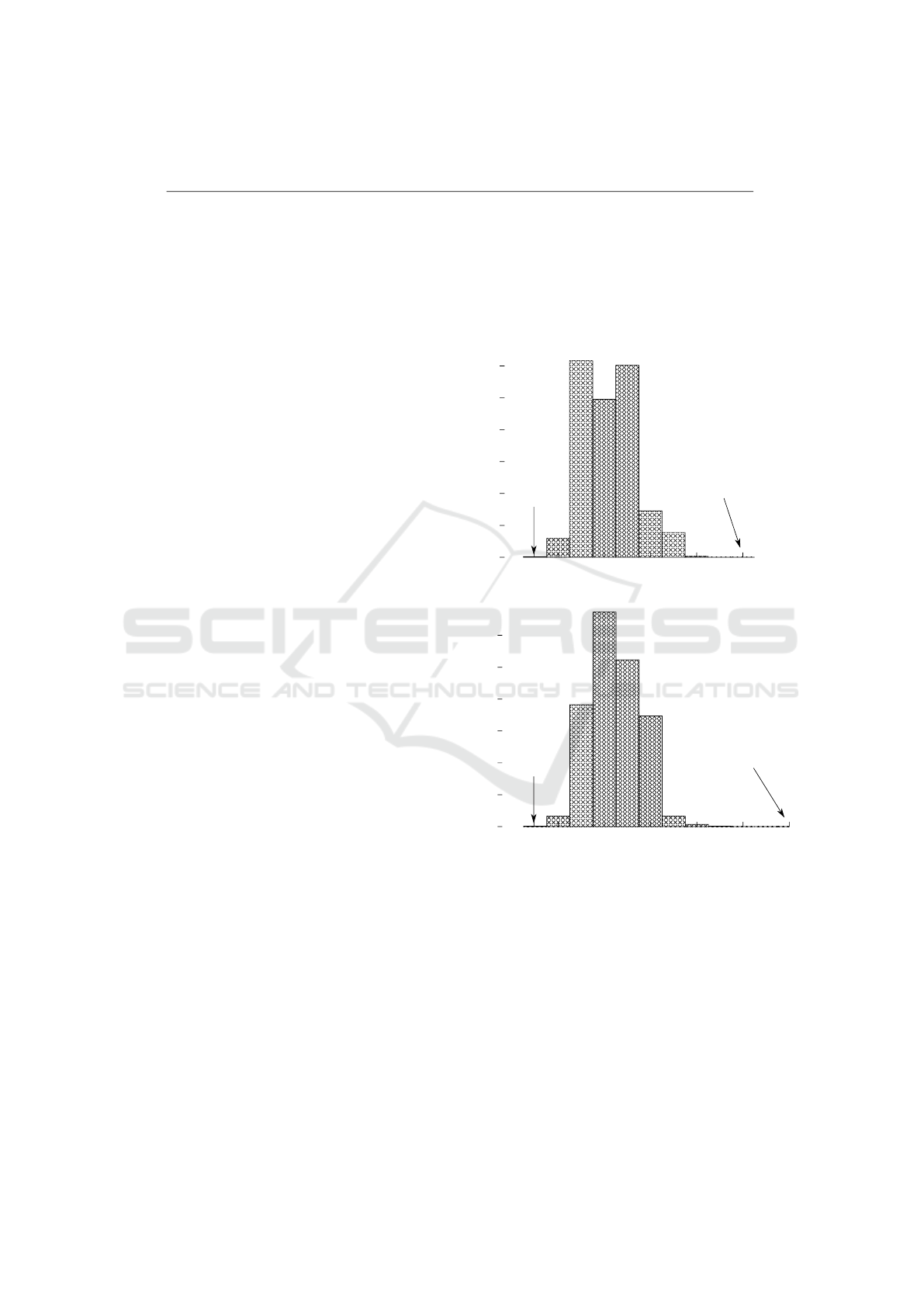
Table 1: Basic graph metrics for Ubuntu releases.
Ubuntu 14.04 Ubuntu 16.04 Ubuntu 18.04 Ubuntu 20.04
Buildable SPKGS 22,028 25,401 28,886 30,646
Full graph edges 207,894 214,982 376,028 387,175
Full graph density 0.0009 0.0007 0.0009 0.0008
Simplified graph vertices 1,646 1,943 1,476 1,770
Simplified graph edges 37,087 45,992 43,363 51,492
Simplified graph density 0.027 0.024 0.040 0.033
This software provides a variety of heuristics, rang-
ing from a simple greedy algorithm to versions that
use heuristics and randomization to find better col-
orings. The programs take input in the “DIMACS
standard format,” as used in the DIMACS challenges
on graph coloring, so our conflict graph construction
software outputs the conflict graphs in this format,
along with a “translation table” that gives the mapping
from each source package name to its corresponding
vertex number.
We first considered two versions of graphs that
represent all source packages, meaning the full con-
flict graph and the simplified version as described in
Section 3.3. We automated the process of running
the coloring algorithms with different random seeds
and different heuristic options, and allowed the col-
oring programs to run for up to a full 24-hour day
on a Linux system with an Intel i7-7700 processor.
For both the full and simplified graphs generated from
the Ubuntu 20.04 distribution, the coloring software
found colorings using as few as 11 colors, meaning
that 11 distinct build environments are sufficient to
build all 30,646 source packages. Since these are
approximation algorithms, we don’t know if 11 is
the minimum possible number of build environments
(or, equivalently, the chromatic number of the conflict
graph), but this is a small number of build environ-
ments for 30,646 packages.
Comparing the performance and success of color-
ing the full graph versus the simplified graph shows
the value of graph simplification: the colorings found
on the simplified graph translate directly to the full
graph, but the reduced size allowed the coloring soft-
ware to run much faster and explore more options
with more random seeds. We completed over a mil-
lion (specifically, 1,050,000) runs on the simplified
graph in 24 hours, while we could only complete
23,835 runs on the full graph. Having a smaller graph
to work with also allowed the heuristic algorithms
to succeed more often, not getting stuck in parts of
the graph that lead to using larger numbers of colors.
Figure 2 shows histograms of the colors found over
all runs, for both the simplified and the full graphs.
Notice that the values are skewed more to the left,
meaning colorings with fewer colors, for the simpli-
Full Graph
0
5
10
15
20
25
30
35
12 14 16
18
20
Simplified Graph
0.08% of runs
give 11 colors
max # colors = 20
11
12 14 16 18 20 22
0.06% of runs
give 11 colors
max # colors = 22
11
0
5
10
15
20
25
30
35
Figure 2: Distribution on number of colors used by heuristic
run, as a percentage of all runs.
fied graph. The range for the simplified graph is also
lower, with the coloring software producing colorings
ranging from 11 to 20 colors on the simplified graph,
and 11 to 22 colors on the full graph.
While the percentage of runs finding the smallest
(11 color) solution is only slightly higher for the sim-
plified graph (0.0806% of runs) than the full graph
(0.0587% of runs), that small advantage coupled with
the much higher rate of testing graphs, means that
the simplified graph found the smallest coloring much
faster than using the full graph. More specifically, the
ICSOFT 2022 - 17th International Conference on Software Technologies
64

first coloring using 11 colors was found in just under
5 minutes on the simplified graph, but an 11-color re-
sult on the full graph was not obtained for an hour and
39 minutes.
4.3 Subgraph Colorings
We next consider finding colorings for nested sub-
graphs, as described in Section 3.2. To construct these
graphs for the Ubuntu 20.04 distribution, we first used
the “Ubuntu Popularity Count” project data to find the
top 500, 1000, 2000, and 4000 source packages. Note
that this is not as simple as just taking the first names
from the popularity count ranking for two reasons:
First, not all packages listed are standard packages in
the Ubuntu release we are interested in (20.04 in this
case), and second, the ranking is for binary packages,
not source packages. To find our lists, we first fil-
tered the popularity contest list to include only binary
packages that are a part of the Ubuntu 20.04 release,
then we mapped binary package names to the source
package used to build that package, and finally we re-
moved all but the first occurrence of each source pack-
age (since a source package can build multiple binary
packages, it is common for multiple binary packages
for the same source package to be in the “Top X”
lists). As a result of this pre-processing, we obtained
a ranked list of source packages used in Ubuntu 20.04
from which we could extract the “Top X” lists.
Next, given the Top 500 source packages, we iden-
tified the vertices in the simplified conflict graph cor-
responding to those packages, removed duplicates,
and then computed the subgraph induced by those
vertices. We repeated this for the top 1000, 2000, and
4000 source packages. Given these graphs, we ran
105,000 iterations of the graph coloring algorithm on
each to determine the smallest coloring we could find
in that amount of time. The results, showing graph
sizes and the best coloring we found, are in Table 2.
We were somewhat surprised at the graph sizes
and densities in the Top 500 and Top 1000 lists. We
initially expected that the main, most popular Ubuntu
packages would share a somewhat similar build envi-
ronment with few conflicts, leaving most conflicts to
arise from more esoteric packages that were less pop-
ular. This turned out not to be the case, with over a
hundred build environments defined even in the small-
est Top 500 list, and a fairly consistent graph density
of 0.02-0.04 in each graph. The colorings we found
do reflect increasing levels of conflicts when more,
less popular packages are included, growing from just
4 colors (build environments) used for the Top 500
and Top 1000 lists, up to the 11 colors required for all
packages.
Due to the small sizes and number of colors found
for the Top 500 and Top 1000 graphs, we performed
another test. Since the size of the maximum clique in
a graph lower-bounds the chromatic number, and we
know the maximum clique of either of these smaller
graphs cannot be more than 4, we performed an ex-
haustive search to find the maximum clique for both
graphs. For the Top 1000 graph, there is indeed a
maximum clique of size 4, so the 4-coloring of the
Top 1000 graph is optimal. However, the maximum
clique in the Top 500 graph has size 3, so it may be
possible to color the Top 500 graph with 3 colors.
Unfortunately, even guaranteeing a small chromatic
number doesn’t allow for efficient, exact optimal col-
oring: The graph coloring problem is NP-complete
even for just distinguishing between 3-colorable and
4-colorable graphs.
As a final note, this project was motivated by our
experience in an earlier project in which we were per-
forming large scale static analysis on the Top 1000
source packages in Ubuntu 18.04. When we ran into
build environment conflicts, we handled this problem
in an ad hoc way, resulting in around a dozen build
environments for the Top 1000 packages. Developing
a formal foundation for creating these build environ-
ments, as we report in this paper, reduces the number
of distinct build environments for that set of package
to just 4 distinct environments. This is a big improve-
ment for both efficiency of performing the analysis,
and for simplicity of managing the 1000 runs of the
static analyzer.
5 RELATED WORK
The public nature of the open-source software com-
munity provides a rich source of data for studying
large software systems. While we are not aware of
any prior work that looks specifically at the prob-
lem we study, defining small sets of build environ-
ments, we briefly survey some of the work related
to analyzing software distributions and dependencies
here. Early studies with Linux distributions, such
as (Gonz
´
alez-Barahona et al., 2003) focused on ba-
sic metrics such as distribution size, package size in
terms of files and lines of code, and programming lan-
guages used. Other studies, such as (Galindo et al.,
2010), used Linux distributions to study general con-
cepts such as variability models for software.
As distributions have grown, the complexity of
dependencies and conflicts have proven to be signif-
icant challenges for package and distribution main-
tainers, and modeling these relations has been studied
formally. (Mancinelli et al., 2006) developed an ex-
Minimum Size Build Environment Sets and Graph Coloring
65

Table 2: Basic graph metrics for Ubuntu 20.04 top-X subgraphs.
Top 500 Top 1000 Top 2000 Top 4000 All SPKGS
Vertices 117 198 355 594 1,770
Edges 151 375 2,388 6,385 51,492
Density 0.022 0.019 0.038 0.036 0.033
Best coloring 4 4 6 7 11
tended graph model that reflects both dependencies
and conflicts, and discussed dependency closures in
ways similar to our work, but with a focus on binary
packages and tasks a maintainer must do to accurately
define and visualize package relations. (de Sousa
et al., 2009) created a similar model, which they use
to study the properties of the dependency graph, look-
ing at degree connectivity distribution and modular-
ity, among other measures. While many of these
works use the Debian distribution due to its popularity
among academics, (Wang et al., 2015) perform simi-
lar graph modeling to visualize package dependencies
in Ubuntu 14.04, although they report only looking at
a graph with 2,240 vertices which would be a small
subset of the total Ubuntu 14.04 packages.
Researchers have also studied dependency and
conflict relations in regard to how changes in pack-
ages can violate relations. (Di Cosmo et al., 2013)
developed a formal model that was used for study-
ing update failures, with a focus on end-users up-
dating their systems as well as maintainers defining
appropriate relations. They look specifically at “co-
installability” of packages, similar to our definition
of compatible build environments, although their fo-
cus is on binary packages and operational systems
rather than build environments. Installability from
an end-user standpoint was also studied by (Vouil-
lon and Cosmo, 2013), where they relate installability
tests to the satisfiability (SAT) problem, bring up NP-
completeness issues as we have, and they also explore
graph simplification/compression techniques similar
to our techniques in Section 3.3. (Claes et al., 2015)
study package conflicts and broken packages at a fine-
grained level, using daily snapshots reflecting ongo-
ing developer work.
Recently, the appearance of language-specific
code repositories for developers, such as NPM (for
JavaScript), CRAN (for R), and PyPI (for Python),
have raised similar dependency challenges, but in a
different context (Decan et al., 2016; Kikas et al.,
2017; Decan et al., 2019). Of particular interest, (De-
can et al., 2016) show that topology of dependency
networks varies between different language ecosys-
tems, and while they did not compare with full operat-
ing system distributions it is a reasonable extension to
believe that the wide diversity of software included in
full operating system distirubions will be even more
different.
The above-mentioned work is focused primarily
on the challenges developers and end users face in
maintaining operational systems in light of dependen-
cies and conflicts, and do not address source packages
or build environments. The only work we’re aware
that looks specifically at large-scale software build-
ing in open source distributions is the work of (Nuss-
baum, 2009), which describes re-building an entire
Debian distribution from source packages. Nussbaum
was interested in whether the “build dependencies”
were defined properly, so created a separate minimal
build environment for each package, and used a large
grid computing infrastructure to perform the builds.
Our work, focused on re-using build environments,
installs far more packages than the minimal set for
any package, so we would not be able to test this par-
ticular feature. We would be able to address another
question tested by Nussbaum, however, and that is the
question of whether updated tool-chains are still capa-
ble of successfully building from the provided source
packages.
6 CONCLUSIONS AND FUTURE
WORK
In this paper, we formalized the problem of design-
ing build environments for large-scale software build-
ing and analyzing, addressing issues with dependen-
cies and conflicts between components. We showed
that there is a one-to-one correspondence between the
problem of minimizing the number of build environ-
ments and the problem of minimizing the number of
colors required to color a constructed graph, which we
call the conflict graph. We also considered ways to
simplify the resulting conflict graph, and considered
the problem of coloring increasing-size nested sub-
graphs. Our results provide some interesting metrics
for the complexity of the build requirements (conflict
graph) for various Ubuntu LTS releases, and we use
heuristic graph coloring software to generate small
numbers of build environments for the Ubuntu 20.04
distribution. We were able to construct a set of 11
build environments that were sufficient to build all
30,646 source packages in Ubuntu 20.04, and a set
ICSOFT 2022 - 17th International Conference on Software Technologies
66

of just 4 environments for building all of the top 1000
“most popular” source packages. The work reported
here provides a clear way to think about the build
environment problem, and the experimental results
show that small sets of build environments are suffi-
cient, significantly improving on the ad hoc approach
to setting up build environments.
There are several directions for future work, and
we describe two immediate open problems here.
First, since dependencies can include disjunctions
(“or-lists”) that can be satisfied in multiple ways,
is there a way to do this that can reduce the num-
ber of build environments? More specifically, our
or-list resolution uses the same process as the stan-
dard Debian build tools, taking the package main-
tainer’s order of the or-list as the priority order for
satisfying the dependency. While this is certainly
a sound approach when making a single build envi-
ronment, when considering build environments sup-
porting multiple packages we may be able to reduce
the number of conflicts by making different choices.
For example, most source packages require either the
pkg-config or pkgconf package, but while pkgconf
is a drop-in replacement for the older pkg-config
some packages keep dependency specifications that
prioritize the older package. Since these two packages
conflict with each other, could forcing all packages to
use pkgconf, despite the package maintainer prior-
ity specification, reduce the number of conflicts and
hence the number of build environments required?
As a second open question, while we studied the
issue of coloring nested subgraphs, we were not able
to formulate a clear objective for this minimization.
Is there a metric for nested subgraph colorings that
makes sense in our setting? The metric may require
some additional information about the efficiency of
performing builds using these environments, or it
might depend on preferences of the users (i.e., priori-
tizing smaller overall number of environments or pri-
oritizing re-use of environments used for subgraphs),
so just determining the proper goal is a first step in
considering algorithms to solve this problem.
REFERENCES
Claes, M., Mens, T., Di Cosmo, R., and Vouillon, J. (2015).
A Historical Analysis of Debian Package Incompati-
bilities. In 2015 IEEE/ACM 12th Working Conference
on Mining Software Repositories, pages 212–223.
de Sousa, O. F., de Menezes M.A., and Penna, T.
(2009). Analysis of the package dependency on De-
bian GNU/Linux. Journal of Computational Interdis-
ciplinary Sciences, 1(2):127–133.
Decan, A., Mens, T., and Claes, M. (2016). On the topol-
ogy of package dependency networks: a comparison
of three programming language ecosystems. In Proc-
cedings of the 10th European Conference on Software
Architecture Workshops (ECSAW), pages 1–4.
Decan, A., Mens, T., and Grosjean, P. (2019). An empirical
comparison of dependency network evolution in seven
software packaging ecosystems. Empirical Software
Engineering, 24(1):381–416.
Di Cosmo, R., Treinen, R., and Zacchiroli, S. (2013). For-
mal Aspects of Free and Open Source Software Com-
ponents. In 11th International Symposium on Formal
Methods for Components and Objects (FMCO), pages
216–239.
Galindo, J., Benavides, D., and Segura, S. (2010). Debian
Packages Repositories as Software Product Line Mod-
els. Towards Automated Analysis. In Proceeding of
the First International Workshop on Automated Con-
figuration and Tailoring of Applications (ACOTA).
Garey, M. R. and Johnson, D. S. (1979). Computers and
intractability. W.H. Freeman, San Francisco.
Gonz
´
alez-Barahona, J. M., Robles, G., Ortu
˜
no-P
´
erez, M.,
Rodero-Merino, L., Centeno-Gonz
´
alez, J., Matell
´
an-
Olivera, V., and Castro-Barbero, E. (2003). Analyzing
the Anatomy of GNU/Linux Distributions: Method-
ology and Case Studies (Red Hat and Debian). In
Free/Open Source Software Development, Idea Group
Inc, pages 27–58.
Jackson, I., Schwarz, C., and Morris, D. A.
(2021). Debian policy manual (version 4.6.0.1).
https://www.debian.org/doc/debian-policy/.
Kikas, R., Gousios, G., Dumas, M., and Pfahl, D. (2017).
Structure and Evolution of Package Dependency Net-
works. In 2017 IEEE/ACM 14th International Confer-
ence on Mining Software Repositories (MSR), pages
102–112.
Mancinelli, F., Boender, J., di Cosmo, R., Vouillon,
J., Durak, B., Leroy, X., and Treinen, R. (2006).
Managing the Complexity of Large Free and Open
Source Package-Based Software Distributions. In 21st
IEEE/ACM International Conference on Automated
Software Engineering (ASE’06), pages 199–208.
Nussbaum, L. (2009). Rebuilding Debian using distributed
computing. In Proceedings of the 7th International
Workshop on Challenges of Large Applications in Dis-
tributed Environments (CLADE), pages 11–16.
The Ubuntu Web Team (2021). Ubuntu popularity contest.
https://popcon.ubuntu.com/.
Vouillon, J. and Cosmo, R. D. (2013). On software compo-
nent co-installability. ACM Transactions on Software
Engineering and Methodology, 22(4):34:1–34:35.
Wang, J., Wu, Q., Tan, Y., Xu, J., and Sun, X. (2015).
A graph method of package dependency analysis on
Linux Operating system. In 2015 4th International
Conference on Computer Science and Network Tech-
nology (ICCSNT), pages 412–415.
Minimum Size Build Environment Sets and Graph Coloring
67
