
A Modified Polynomial Preserving Recovery Technique
M. Barakat
1,2 a
, W. K. Zahra
1,3 b
and A. Elsaid
1,4 c
1
Department of Mathematics, Institute of Basic and Applied Sciences,
Egypt-Japan University of Science and Technology (E-JUST), New Borg El-Arab City, Alexandria, Egypt
2
Department of Basic Engineering Sciences, Faculty of Engineering, Menofia University, Shebin El-Kom, Egypt
3
Department of Engineering Physics and Mathematics, Faculty of Engineering, Tanta University, Tanta, Egypt
4
Department of Mathematics and Engineering Physics, Faculty of Engineering, Mansoura University, Mansoura, Egypt
Keywords:
Finite Element Method, Modified Polynomial Preserving Recovery, Gradient Recovery Technique.
Abstract:
In this work, the polynomial preserving recovery method is enhanced by increasing the order of the fitting
polynomial within the same patch. This is achieved by adding more sample points inside the elements of the
patch then substitute them in the discretized form of the differential equation. These sample points are the
set of superconvergent points of the patch under consideration. Numerical results show that the recovered
gradient at the nodes with linear elements is superconvergent. The proposed method improves the accuracy of
the recovered gradient over the domain of the solution with the same rate of convergence of the polynomial
preserving recovery technique.
1 INTRODUCTION
Gradient recovery techniques are post-processing
methods in which the finite element solution is uti-
lized to build a recovered gradient. Several techniques
were developed as in (Levine, 1985) and (Bramble
and Schatz, 1977), but they suffered from long execu-
tion time, complexity, requiring special mesh struc-
ture, or the necessity of using low order finite ele-
ments. The super-convergent patch recovery (SPR)
technique or the ZZ recovery technique (Zienkiewicz
and Zhu, 1992) was the first method to overcome
these obstacles. The SPR has been introduced to re-
cover the accuracy and continuity in the gradient field.
The method least-squares fits the stresses at super-
convergent points or points whose accuracy is high on
element patches (Barlow, 1976) to obtain the gradient
at the nodes. The super-convergence properties of the
SPR are proved in (Li and Zhang, 1999) and (Zhang,
2000), and the efficiency of the ZZ error estimator is
presented in (Ainsworth et al., 1989). Several treat-
ments to improve the recovered gradient of the SPR
have been proposed. The authors in (Blacker and Be-
lytschko, 1994) improved the accuracy of the gradi-
a
https://orcid.org/0000-0003-0897-1752
b
https://orcid.org/0000-0002-6448-6877
c
https://orcid.org/0000-0002-8248-3119
ents by including the squares of the residuals of the
equilibrium equations and the boundary conditions.
They introduced a new conjoint polynomial for inter-
polating the stresses of the local patch to improve the
projection scheme. Li and Wiberg (Li and Wiberg,
1994) fitted a higher order polynomial expansion to
the finite element solution at super-convergent points
in a patch of elements that include the targeted ele-
ment and its neighbors. Wiberg et al. (Wiberg et al.,
1994) proposed an enhancement of the SPR for lin-
ear elasticity problems and achieved an improvement
in the gradient recovery near the boundaries. Gu et
al. (Gu et al., 2004) modified the SPR for the nonlin-
ear problems by using integration points as sampling
points, applying weighted average procedure, and in-
troducing additional nodes.
Zhang and Naga (Zhang and Naga, 2005) and
(Naga and Zhang, 2005) introduced the polynomial
preserving recovery (PPR) method. The idea of the
method starts by constructing a patch of elements
around a targeted node. Then the numerical solu-
tion at the nodes of the patch is fitted to a polyno-
mial one degree higher than the solution. The fit-
ting polynomial is differentiated to obtain the gradi-
ent at the node. The PPR was also employed to im-
prove eigenvalue approximation (Naga et al., 2006)
and (Shen and Zhou, 2006). In (Guo et al., 2016), the
authors provided two strategies to enhance the gradi-
Barakat, M., Zahra, W. and Elsaid, A.
A Modified Polynomial Preserving Recovery Technique.
DOI: 10.5220/0011263400003274
In Proceedings of the 12th International Conference on Simulation and Modeling Methodologies, Technologies and Applications (SIMULTECH 2022), pages 63-69
ISBN: 978-989-758-578-4; ISSN: 2184-2841
Copyright
c
2022 by SCITEPRESS – Science and Technology Publications, Lda. All rights reserved
63

ent at the boundaries. The study of the PPR was gen-
eralized to high frequency wave problems (Guo and
Yang, 2017). The recovered gradient of the PPR is
also used in adaptive refinement for Fredholm inte-
gral equation (Adel et al., 2016). The PPR is used to
recover the heat flux for skin tissues in the presence
of a tumor (Essam et al., 2019).
In this paper, we propose a modification to the
PPR technique. Our modified technique builds a so-
lution of a higher order polynomial within the same
patch of the classical PPR. We substitute sample
points within the elements of the patch in the dis-
cretized form of the differential equation. The sam-
ple points chosen in this work are the superconvergent
points used in the SPR method. Then the resultant
system of equations together with the system resulting
from the PPR are solved together in the least-squares
sense to evaluate the coefficients of our solution. Fi-
nally, the higher order solution is differentiated to get
the gradient at the desired node.
The rest of the paper is organized as follows. In
section 2, the basic concepts of the PPR are intro-
duced. The proposed technique is presented in sec-
tion 3. Section 4 contains some numerical examples
to validate the accuracy and the robustness of the pro-
posed technique. Finally, the findings of this work are
summarized in section 5.
2 THE PPR METHOD
We firstly give some notations and review the basic
concepts of the PPR method introduced in (Naga and
Zhang, 2005) and (Zhang and Naga, 2005).
Let v denote a vertex in a finite element mesh, n
be a positive integer, and `(v, n) denote the union of
the elements in the first n layers around v, i.e.,
`(v,n) :=
[
{τ : τ ∈ τ
h
, τ ∩ `(v, n − 1) 6=
/
0}, (1)
where τ is an element in a finite element triangulation
τ
h
and `(v,0) := {v}.
Let N
h
denote all the mesh nodes and V
h
be a fi-
nite element space of degree m over the triangulation
τ
h
. The standard Lagrange basis of V
h
is denoted by
{φ
v
: v ∈ N
h
}. The PPR gradient recovery operator
is denoted by G
h
such that G
h
: V
h
−→ V
h
×V
h
. For
a mesh node v, a patch of elements around v is de-
noted by α
v
. To recover the gradient at v, a polyno-
mial p
v
∈ P
m+1
(α
v
) is to be fitted in the least-square
sense using the set of nodes N
h
∩ α
v
, i.e.
p
v
= arg min
p∈P
m+1
(α
v
)
∑
v∈N
h
∩α
v
(u
h
− p)
2
(v), (2)
where P
m+1
(α
v
) is the space of all polynomials de-
fined on the patch α
v
with degree less than or equal
m + 1. Then the gradient at the node v is given by
(G
h
u
h
)(v) = ∇p
v
(v). (3)
After getting the gradient at all vertices, we utilize in-
terpolation with the original basis function of V
h
to
evaluate the gradient representation over the whole
domain as
(G
h
u
h
) :=
∑
v∈N
h
(G
h
u
h
)(v)φ
v
. (4)
For an interior node v we define α
v
as the small-
est `(v, n) that ensures the uniqueness of the fitting
polynomial (Naga and Zhang, 2005) and (Zhang and
Naga, 2005). In the case that v is a boundary node,
consider r to be the smallest positive integer to ensure
that `(v, r) has at least one interior mesh node. Then,
we define
α
v
= `(v, r) ∪ {α
˜v
: ˜v ∈ `(v,r) : and ˜v an interior
vertex}.
(5)
The superconvergence analysis of G
h
in (Zhang and
Naga, 2005) showed that if u ∈ W
m+2
∞
(α
v
), then
k∇u − G
h
u
h
k
L
∞
(α
v
)
6 Ch
m+1
|u|
W
m+2
∞
(α
v
)
. (6)
where the PPR operator G
h
preserves polynomials of
degrees up to m + 1 in the domain.
3 MODIFIED PPR METHOD
We refer to the proposed recovery technique as
(MPPR). The objective of this method is to construct
an enhanced recovered gradient (G
h
u
h
) at each node
then use them to get a recovered gradient over the do-
main by interpolation. This method is only applica-
ble when the source term f can be evaluated at any
point in the domain. To recover the gradient at a
node v, we assume that the solution over the patch
of this node is a high order polynomial p
m
(x). We
use two sets of sampling points to determine the co-
efficients of this polynomial. The first set contains
inner-element points inside the patch. The points of
this set are substituted in the discretized form of the
differential equation. We choose these points to be
the superconvergent points or the points whose finite
element stress is of high accuracy. Then we follow
the same steps of the classical PPR to get the other
set which consists of the nodes of the patch. Finally,
we get a system of algebraic equations that we solve
in the least-squares sense to get the desired coeffi-
cients. If the nodes N
h
∩ α
v
from the first patch α
v
together with inner-element nodes are not enough for
the uniqueness condition of the desired polynomial,
SIMULTECH 2022 - 12th International Conference on Simulation and Modeling Methodologies, Technologies and Applications
64

we go further to include the nodes from the follow-
ing patch. We keep this process until the uniqueness
condition is met.
In this work, for the one-dimensional case, we
consider the following differential equation
L(u(x)) = f (x); x ∈ Ω. (7)
We construct a polynomial of an order m (higher than
the order of the finite element solution) p
m
(x) that ap-
proximates the solution u(x) of the considered prob-
lem.
p
m
(x) = Pa, (8)
where
P = (1, x, x
2
,..., x
m
), a
T
= (a
0
, a
1
, a
2
,..., a
m
). (9)
We consider an interior node v and its patch α
v
. Then,
for all the nodes ϑ in N
h
∩ α
v
, we have
p
m
(x
ϑ
) = u
h
(x
ϑ
), (10)
where x
ϑ
are the coordinates of the nodes ϑ of the
patch
Then we substitute the polynomial p
m
in the differen-
tial equation to evaluate
L(p
m
(x
j
)) = f (x
j
). (11)
where x
j
are the coordinates of the superconvergent
points inside the elements of the patch
We solve this system of equations to obtain the co-
efficients of the polynomial p
m
. Then the recovered
gradient at the node v is given by
(G
h
u
h
)(v) =
d
dx
(p
m
(v)), (12)
The recovered gradient over the entire domain is ob-
tained using the original shape function as
G
h
u
h
=
∑
v∈N
h
(G
h
u
h
)(v)φ
v
. (13)
3.1 Adaptive Refinement
Adaptive refinement based on an a posteriori error es-
timator is widely used in FEMs. It is proved to be
a useful tool for reducing the computational cost of
solving differential equations as the refinement is di-
rected toward regions where the solution is of a low
quality. The new operator G
h
u
h
is tested as an er-
ror estimator in an adaptive FEM algorithm. The
main steps of the algorithm are solving, estimating
then refining. The considered differential equation is
solved using FEM with linear elements. The recov-
ered gradient obtained by the MPPR is calculated at
each node. Then the refinement process is controlled
by the following estimator:
e = kG
h
u
h
− ∇u
h
k.
This estimator is evaluated at each element. All
elements where the estimator exceeds a prescribed
value are refined. We keep this process till the stop-
page criterion is satisfied.
4 NUMERICAL RESULTS
In this section, we solve various problems using lin-
ear finite element method to illustrate the efficiency
of the proposed approach. The fitting polynomial is
chosen to be of a fourth order. The first two examples
compare the new technique to the PPR over uniform
refinement. We define the L
∞
norm error as the maxi-
mum error at the inner nodes. The other two examples
test the gradient operator of the proposed technique
as an a posteriori error estimator for adaptive refine-
ment.
Example 1 (Zienkiewicz and Zhu, 1992): Consider
the 1D linear differential equation
−
d
dx
du
dx
+ u = f ; x ∈ (0, 1),
with boundary conditions
u(0) = 0, u(1) = 0,
where the function f (x) is chosen so that the exact
solution is given by
u(x) = x
2
−
sinh4x
sinh4
.
Figures (1) and (2) show a comparison of the errors
between the exact gradient and the recovered gradient
obtained using PPR and MPPR methods in L
∞
and L
2
norms, respectively. The MPPR technique yields bet-
ter results than those obtained by the standard PPR
technique. Using the same original basis function
to construct the new gradient affects the error in L
2
norm. The new method keeps the same order of con-
vergence of the PPR
The values of G
h
u
h
and G
h
u
h
together with the exact
gradient over the entire domain are plotted in figure
(3) for four linear elements. The nodal values of the
recovered gradient obtained by the MPPR are better
than those obtained by the PPR. It is apparent that the
proposed approach performs better at the boundaries
of the domain.
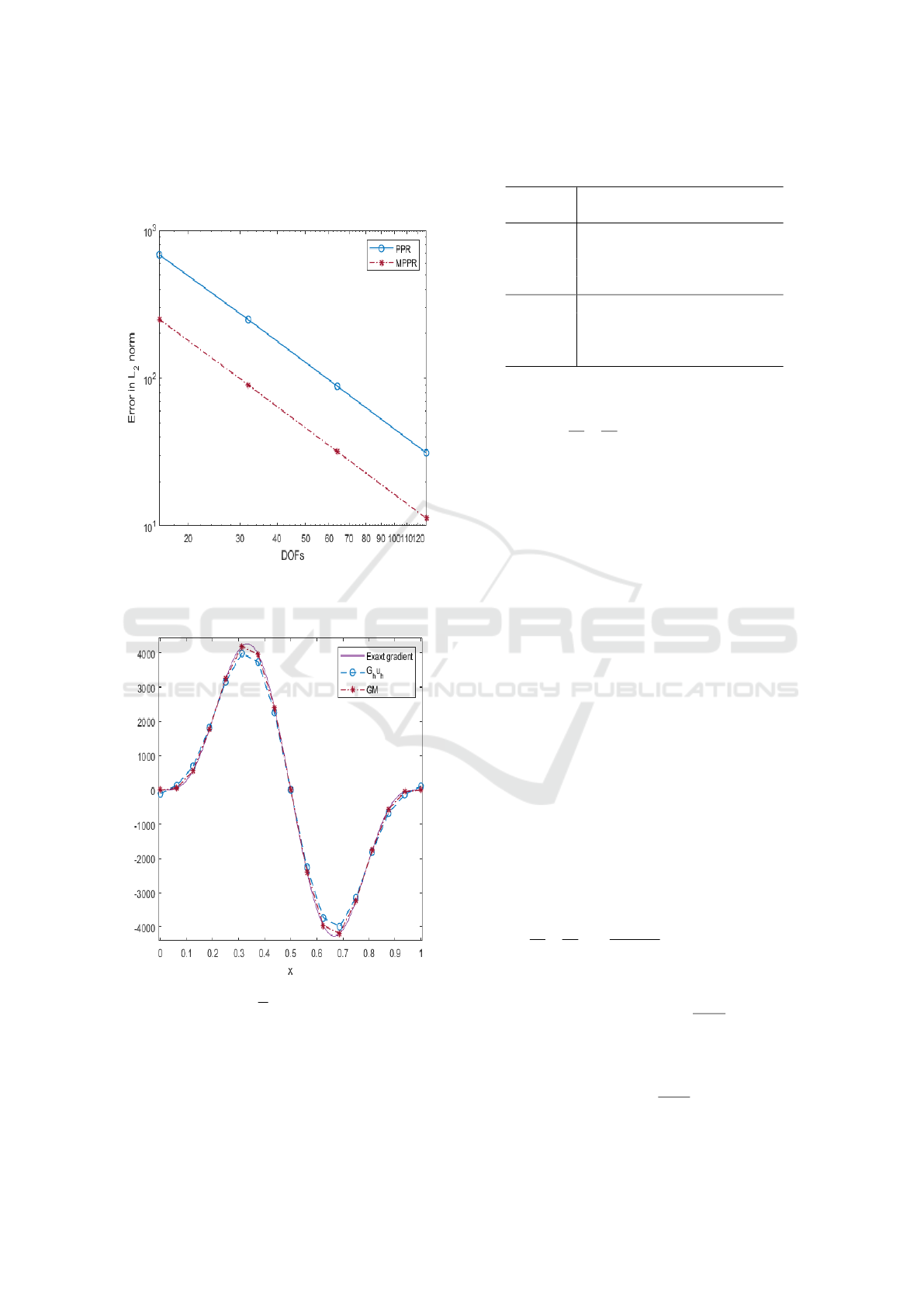
Example 2 (Mitchell, 2013): Consider the 1D linear
differential equation
−
d
dx
du
dx
= f ; x ∈ (0,1),
A Modified Polynomial Preserving Recovery Technique
65
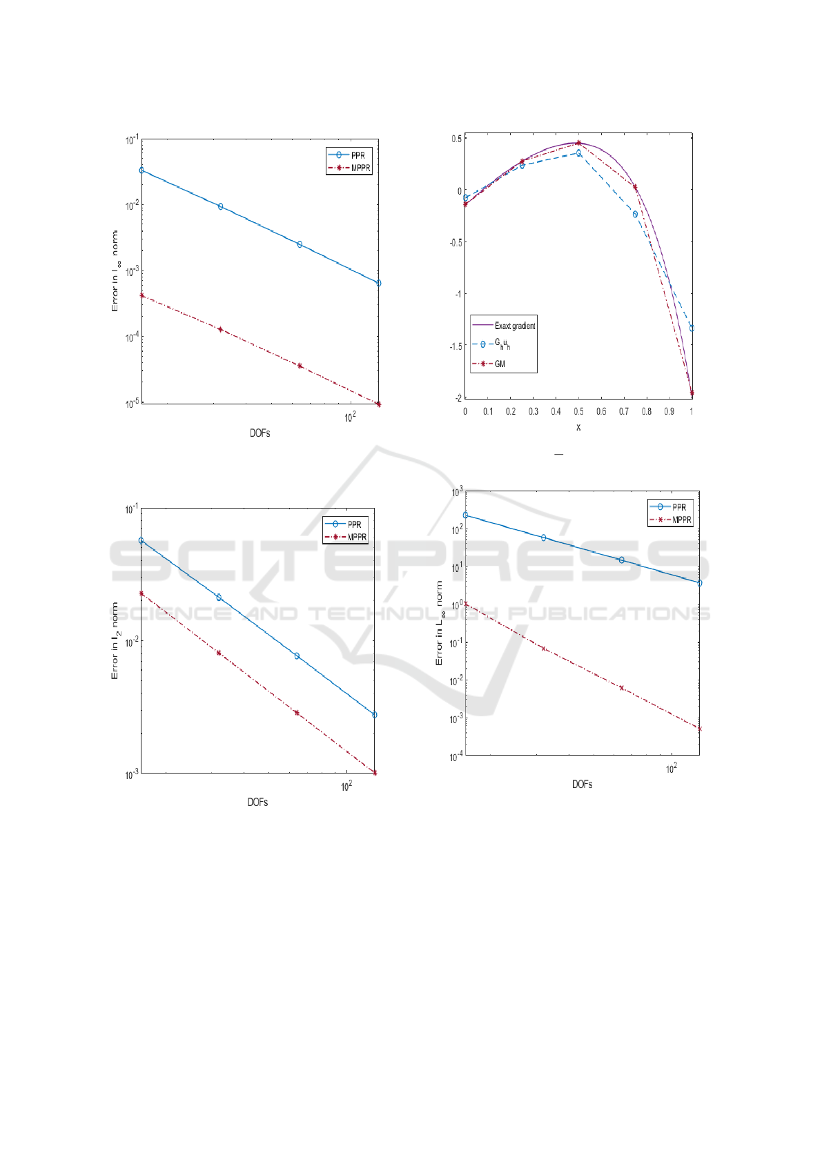
Figure 1: The L
∞
norm error between the exact gradient
and the recovered gradients obtained by by the PPR and the
MPRR for example (1).
Figure 2: The L
2
norm error between the exact gradient and
the recovered gradient obtained by the PPR and the MPRR
for example (1).
with boundary conditions
u(0) = 0, u(1) = 0,
where the function f (x) is chosen so that the exact
solution is given by
u(x) = 2
2a
x
a
(1 − x)
a
.
The given problem is well behaved with no singular-
ities where PPR can perform well. For a = 10, fig-
Figure 3: Distribution of the exact gradient and the recov-
ered gradients G
h
u
h
and (G
h
u
h
) of example (1).
Figure 4: The L
∞
norm error between the exact gradient and
the recovered gradients obtained by the PPR and the MPRR
for example (2).
ure (4) and figure (5) clarify that the MPPR method
presents leading results to the PPR in both norms.
Again, the same order of convergence of the PPR is
preserved in the proposed technique.
Figure (6) shows a comparison between the recovered
gradients and the exact one over 16 linear elements.
The accuracy of the gradient of the MPRR is higher
than that of the PPR especially at the nodes.
Table (1) shows a comparison between the average
SIMULTECH 2022 - 12th International Conference on Simulation and Modeling Methodologies, Technologies and Applications
66
computing time of both methods for examples (1) and
(2). The MPPR takes slightly longer time to compute
the gradient.
Figure 5: The L
2
norm error between the exact gradient and
the recovered gradient obtained by the PPR and the MPRR
for example (2).
Figure 6: Distribution of the exact gradient and the recov-
ered gradients G
h
u
h
and (G
h
u
h
) of example (2).
The author in (Mitchell, 2013) made a collec-
tion of problems for testing adaptive refinement tech-
niques. We utilize two of these problems to show the
efficiency of the new operator as an error estimator in
adaptive refinement algorithm.
Table 1: Comparison between average computing time of
the PPR and the MPPR.
DOFs
average time (sec.)
PPR MPPR
Example
(1)
16 0.19 0.23
32 0.38 0.45
64 0.74 0.87
128 1.43 1.69
Example
(2)
16 0.19 0.22
32 0.36 0.43
64 0.73 0.88
128 1.44 1.68
Example 3: Consider the 1D linear differential equa-
tion
−
d
dx
du
dx
= f ; x ∈ (0,1),
with boundary conditions
u(0) = exp(−µ(x
c
)
2
), u(1) = exp(−µ(1 − x
c
)
2
),
where the function f (x) is chosen so that the exact
solution is given by
u(x) = exp(−µ(x − x
c
)
2
),
where 0 < x
c
< 1.
This problem has an exponential peak inside the do-
main of its solution. The location of the peak is at
x = x
c
, and the strength of the peak depends on the
parameter µ.
We use the L
2
norm error between the finite ele-
ment gradient and the recovered gradient from the two
methods as an error estimator. In each case, we evalu-
ate the L
2
norm error between this recovered gradient
and the exact gradient. Results for different values of
µ and x
c
= 0.5 are presented in Figure (7) and figure
(8). It is apparent that the grids resulting when apply-
ing the two methods in adaptive refinement are very
close. Results emphasize the superiority of the pro-
posed technique over the PPR regarding the accuracy
of the gradient.
Example 4: Consider the Helmholtz equation
−
d
dx
du
dx
−
1
(λ + x)
4
u = f ; x ∈ (0,1),
with boundary conditions
u(0) = 0, u(1) = sin
1
λ + 1
,
where the function f (x) is chosen so that the exact
solution is given by
u(x) = sin
1
λ + x
.
A Modified Polynomial Preserving Recovery Technique
67
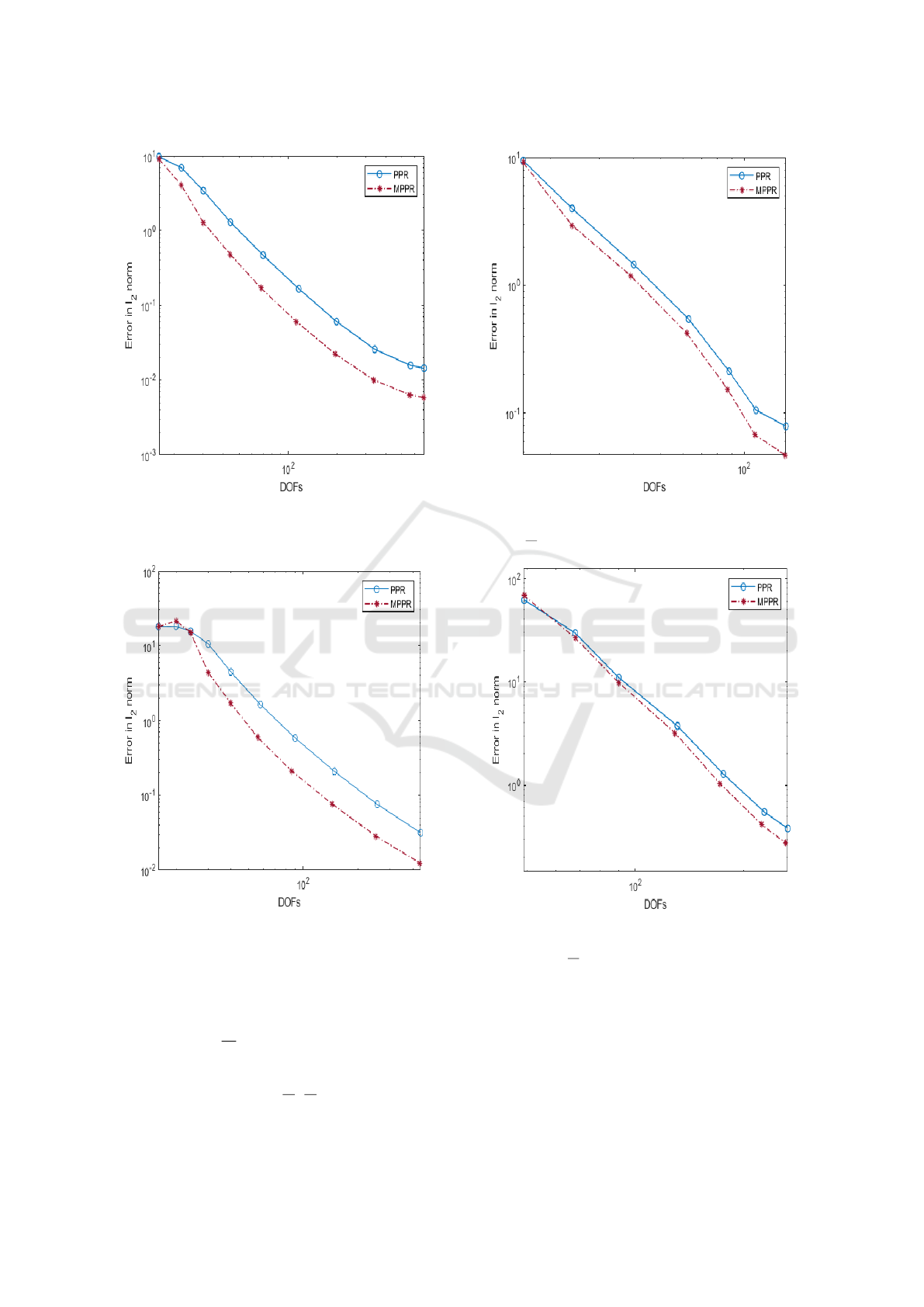
Figure 7: The L
2
norm error between the exact gradient and
the recovered gradient obtained by the PPR and the MPRR
for µ = 10
3
for example (3).
Figure 8: The L
2
norm error between the exact gradient and
the recovered gradient obtained by the PPR and the MPRR
for µ = 10
4
for example (3).
This problem exhibits an oscillatory behaviour
near the origin where the wavelength decreases. The
number of the oscillations N depends on the parame-
ter λ, where λ =
1
Nπ
.
The error between the exact gradient and the re-
covered gradients in the L
2
norm form is presented in
figures (9) and (10) for λ =
1
2π
,
1
4π
respectively. Again,
we can see that the results obtained by the MPPR ap-
Figure 9: The L
2
norm error between the exact gradient and
the recovered gradients obtained by the PPR and the MPRR
for λ =
1
2π
for example (4).
Figure 10: The L
2
norm error between the exact gradient
and the recovered gradients obtained by the PPR and the
MPRR for λ =
1
4π
for example (4).
proach are preferable to those obtained by the classi-
cal PPR method.
SIMULTECH 2022 - 12th International Conference on Simulation and Modeling Methodologies, Technologies and Applications
68

5 CONCLUSION
An modified PPR technique is presented. The main
idea is to increase the order of the fitting polynomial
without including other patches. To achieve that, sam-
ple points are substituted in the discretized form of the
differential equation. The sample points are chosen to
be the superconvergent points in the considered patch.
The proposed technique benefits from the high or-
der of the polynomial capturing oscillations and rapid
changes in the solution. It also keeps the local behav-
ior of the solution around the targeted node. The new
operator of the proposed method is also used as an a
posteriori error estimator in adaptive refinement.
Numerical results show that the accuracy of the
new recovered gradient is higher than that obtained
with the PPR and that the proposed method keeps the
same order of convergence as the PPR.
Our future goals are to extend our method to the
higher-dimensional cases and perform a convergence
analysis of the new operator. We also aim to develop
an approach for choosing the inner-elements points
to achieve the best accuracy.
ACKNOWLEDGMENT
This work is supported by the Missions Sector of
the Ministry of Higher Education (MoHE) in Egypt
through an M.Sc. scholarship.
REFERENCES
Adel, E., Elsaid, A., and El-Agamy, M. (2016). Adaptive
finite element method for fredholm integral equation.
South Asian J.
Ainsworth, M., Zhu, J. Z., Craig, A. W., and Zienkiewicz,
O. C. (1989). Analysis of the zienkiewicz–zhu a-
posteriori error estimator in the finite element method.
International Journal for numerical methods in engi-
neering, 28(9):2161–2174.
Barlow, J. (1976). Optimal stress locations in finite element
models. International Journal for Numerical Methods
in Engineering, 10(2):243–251.
Blacker, T. and Belytschko, T. (1994). Superconvergent
patch recovery with equilibrium and conjoint inter-
polant enhancements. International Journal for Nu-
merical Methods in Engineering, 37(3):517–536.
Bramble, J. H. and Schatz, A. H. (1977). Higher order local
accuracy by averaging in the finite element method.
Mathematics of Computation, 31(137):94–111.
Essam, R., El-Agamy, M., and Elsaid, A. (2019). Heat flux
recovery in a multilayer model for skin tissues in the
presence of a tumor. The European Physical Journal
Plus, 134(6):285.
Gu, H., Zong, Z., and Hung, K. (2004). A modified su-
perconvergent patch recovery method and its applica-
tion to large deformation problems. Finite Elements
in Analysis and Design, 40(5-6):665–687.
Guo, H. and Yang, X. (2017). Polynomial preserving re-
covery for high frequency wave propagation. Journal
of Scientific Computing, 71(2):594–614.
Guo, H., Zhang, Z., Zhao, R., and Zou, Q. (2016). Poly-
nomial preserving recovery on boundary. Journal of
Computational and Applied Mathematics, 307:119–
133.
Levine, N. (1985). Superconvergent recovery of the gra-
dient from piecewise linear finite-element approxima-
tions. IMA Journal of numerical analysis, 5(4):407–
427.
Li, B. and Zhang, Z. (1999). Analysis of a class of super-
convergence patch recovery techniques for linear and
bilinear finite elements. Numerical Methods for Par-
tial Differential Equations: An International Journal,
15(2):151–167.
Li, X. and Wiberg, N.-E. (1994). A posteriori error esti-
mate by element patch post-processing, adaptive anal-
ysis in energy and l2 norms. Computers & structures,
53(4):907–919.
Mitchell, W. F. (2013). A collection of 2d elliptic problems
for testing adaptive grid refinement algorithms. Ap-
plied mathematics and computation, 220:350–364.
Naga, A. and Zhang, Z. (2005). The polynomial-preserving
recovery for higher order finite element methods in 2d
and 3d. Discrete & Continuous Dynamical Systems-B,
5(3):769.
Naga, A., Zhang, Z., and Zhou, A. (2006). Enhancing
eigenvalue approximation by gradient recovery. SIAM
Journal on Scientific Computing, 28(4):1289–1300.
Shen, L. and Zhou, A. (2006). A defect correction scheme
for finite element eigenvalues with applications to
quantum chemistry. SIAM Journal on Scientific Com-
puting, 28(1):321–338.
Wiberg, N.-E., Abdulwahab, F., and Ziukas, S. (1994).
Enhanced superconvergent patch recovery incorporat-
ing equilibrium and boundary conditions. Interna-
tional Journal for Numerical Methods in Engineering,
37(20):3417–3440.
Zhang, Z. (2000). Ultraconvergence of the patch re-
covery technique ii. Mathematics of Computation,
69(229):141–158.
Zhang, Z. and Naga, A. (2005). A new finite element gra-
dient recovery method: superconvergence property.
SIAM Journal on Scientific Computing, 26(4):1192–
1213.
Zienkiewicz, O. C. and Zhu, J. Z. (1992). The superconver-
gent patch recovery and a posteriori error estimates.
part 1: The recovery technique. International Journal
for Numerical Methods in Engineering, 33(7):1331–
1364.
A Modified Polynomial Preserving Recovery Technique
69
