Neural Networks for Indoor Localization based on Electric Field Sensing

Florian Kirchbuchner

1 a

, Moritz Andres

2 b

, Julian von Wilmsdorff

and Arjan Kuijper

1 c

Fraunhofer IGD Darmstadt, Fraunhoferstrasse 5, Darmstadt, Germany

Technische Universit

at Darmstadt, Germany

Keywords:

Localization, Indoor Localization, Electronic Field Sensing, Neural Networks, Machine Learning, Data

Acquisition.

Abstract:

In this paper, we will demonstrate a novel approach using artiﬁcial neural networks to enhance signal process-

ing for indoor localization based on electric ﬁeld measurement systems Up to this point, there exist a variety

of approaches to localize persons by using wearables, optical sensors, acoustic methods and by using Smart

Floors. All capacitive approaches use, to the best of our knowledge, analytic signal processing techniques to

calculate the position of a user. While analytic methods can be more transparent in their functionality, they

often come with a variety of drawbacks such as delay times, the inability to compensate defect sensor inputs or

missing accuracy. We will demonstrate machine learning approaches especially made for capacitive systems

resolving these challenges. To train these models, we propose a data labeling system for person localization

and the resulting dataset for the supervised machine learning approaches. Our ﬁndings show that the novel

approach based on artiﬁcial neural networks with a time convolutional neural network (TCNN) architecture

reduces the Euclidean error by 40% (34.8cm Euclidean error) in respect to the presented analytical approach

(57.3cm Euclidean error). This means a more precise determination of the user position of 22.5cm centimeter

on average.

1 INTRODUCTION

In the ﬁeld of ambient assisted living, or AAL for

short, localization of an user is a key role of sensor

functionality. Many technologies capable of indoor

localization already found their way into our daily life

with the rise of smart homes. The applications are

numerous and range from navigation of indoor clean-

ing devices, such as automated vacuum cleaners, se-

curity applications like burglar detection and various

energy optimization tasks. The latter can be achieved

by controlling lights and heaters in a more granular

way, since these resource intensive actors are mostly

needed near the position of a person.

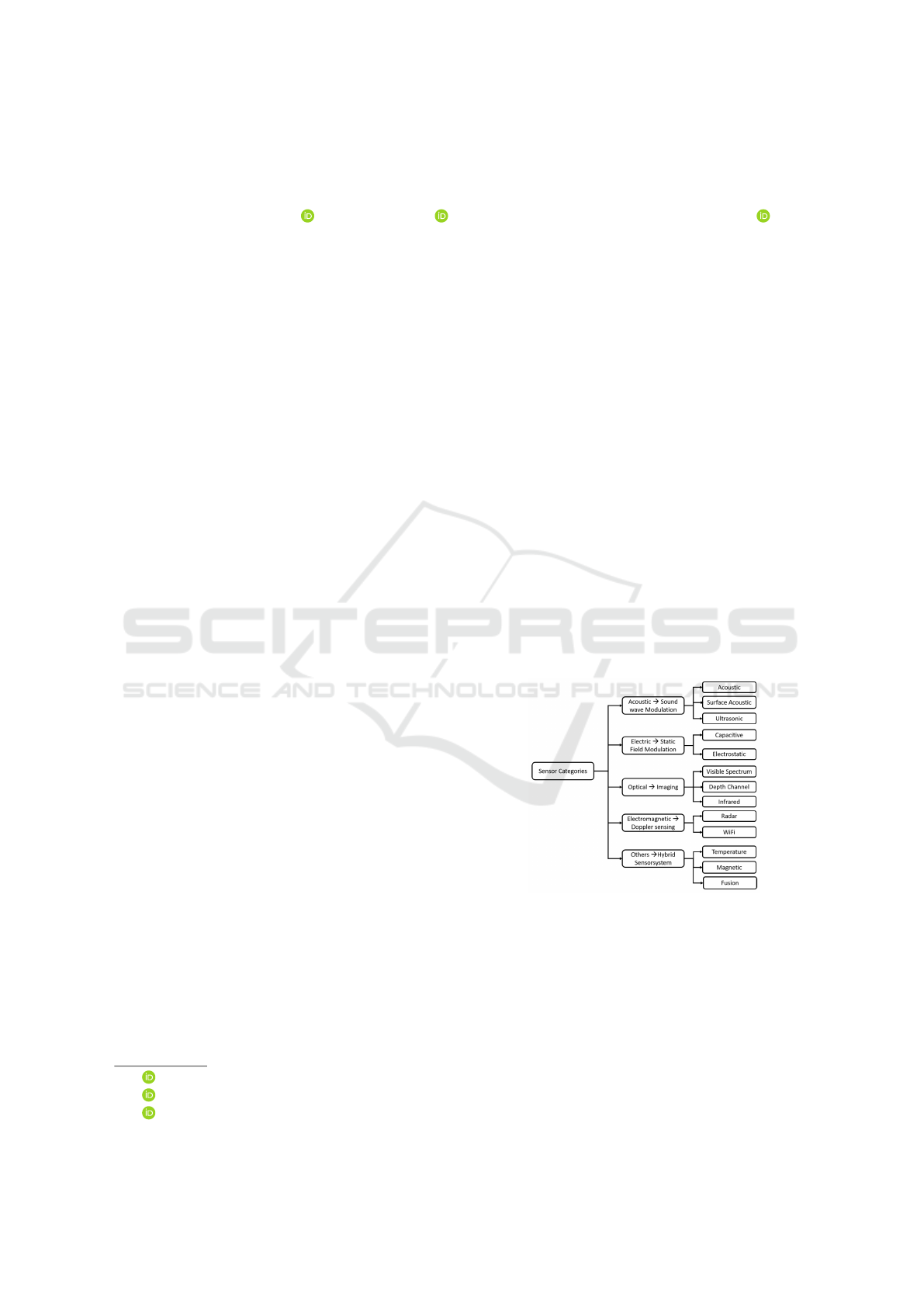
There are numerous solutions for indoor localiza-

tions. Fu et al. (Fu et al., 2020a) have classiﬁed the

sensor categories into acoustic, electric, optical, elec-

tromagnetic and hybrid systems. A deeper view is

given in Figure 1.

Currently, there are many publications on wire-

less localization solutions in the literature. Machine

https://orcid.org/0000-0003-3790-3732

https://orcid.org/0000-0001-6115-5098

https://orcid.org/0000-0002-6413-0061

Figure 1: Sensor categorization for indoor localization as

depicted by Fu et al.(Fu et al., 2020a).

learning methods are often used in this context. Obei-

dat et al. considered satellite-based, magnetic-based,

sound-based optical-based and RF-based technolo-

gies (Obeidat et al., 2021). The presented approaches

mainly operate in the 2.4GHz region and locate the

person using the angle of arrival, time of arrival as

well as by using the received signal strength. Also

Roy et al. summarized similar technologies for indoor

localization mainly based on wireless systems such as

WiFi, Infrared, RFID, Bluetooth and more(Roy and

Kirchbuchner, F., Andres, M., von Wilmsdorff, J. and Kuijper, A.

Neural Networks for Indoor Localization based on Electric Field Sensing.

DOI: 10.5220/0011266300003277

In Proceedings of the 3rd International Conference on Deep Learning Theory and Applications (DeLTA 2022), pages 25-33

ISBN: 978-989-758-584-5; ISSN: 2184-9277

Chowdhury, 2021). The authors focused on tech-

nologies using machine learning techniques, but in

contrast to our approach, none of them use capaci-

tive sensors in combination with machine learning ap-

proaches.

As shown, many systems rely on some sort of time

of ﬂight or other optical solutions. While many of

these optical systems provide a superb resolution and

are robust for indoor localization, they lack a very im-

portant property - user acceptance.

As shown by Kirchbuchner et al. (Kirchbuchner

et al., 2015) most people have less concerns using a

smart ﬂoor system than using an equivalent localiza-

tion system based on cameras.

Frank et al. showed similar results in a conducted

survey(Frank and Kuijper, 2020). Although he pri-

marily considered capacitive sensors for the use in au-

tomotive systems, his results can be generalized.

A reason for the lack of machine learning ap-

proaches for indoor localization with capacitive sys-

tem could be the large amount of data that is required

to train such a system. Since there are no datasets

for these kind of problems because capacitive sys-

tems and their recorded data have not been standard-

ized in any shape of form, Fu et al. also published

approaches to augment time series of capacitive data

sets(Fu et al., 2020b). With this, datasets of capacitive

data can be artiﬁcially enlarged to improve training

results.

As described by Nam et al., some efforts have

been made to integrate machine learning techniques

in capacitive screen technologies(Nam et al., 2021).

These approaches were used to improve the sensing

performance of the devices, to discriminate individ-

ual touches and for user identiﬁcation as well as au-

thentication. But as mentioned, these approaches use

systems with a much higher resolution.

Faulkner et al. closes the gap between capaci-

tive touch systems and indoor localization by present

a very ﬁne granular localization approach(Faulkner

et al., 2020) - with the drawback of using a lot of

computing power to cover a small spacial area with

sensors. Faulkner et al. want to use machine learn-

ing as described in their future work section, but not

for the localization itself. But this case is particularly

interesting because it could lead to localization sys-

tems with a higher resolution and the need of less sen-

sors, which would lead to enormous savings in cost

for such an indoor localization system.

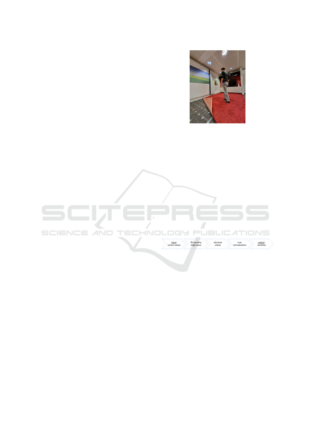
Figure 2: Test person walking on smart ﬂoor with visible

wire pattern.

2 OWN APPROACH

In this chapter we will describe the methods for the

person localization. First, we describe the analytical

approach which has been used up to now with an error

of 57.3cm. Afterwards, we will present the artiﬁcial

neural networks and show that these models are supe-

rior to the previous technique.

2.1 Analytic Approach

For our analytic method we used multi-staged pre-

processing pipeline for each sensor depicted in ﬁgure

3 and a heatmap pipeline as shown in ﬁgure 6.

Figure 3: Processing pipeline for each signal from the EFS

sensors.

The ﬁrst stage of the pre-processing pipeline is

a high pass ﬁlter which removes the value drift of

the sensors and therefore helps to identify true sen-

sor activities. This is necessary since passive electric

ﬁeld sensors (also called electric potential sensors) are

prone to distortions arising from the ambient electri-

cal 50Hz ﬁeld, which occurs in every building from

the in-cooperated power-lines. The drift of these sen-

sors results from an aliasing effect when sampling this

nearly 50Hz ambient sine wave with a nearly 50Hz

clock. For this purpose we use a fast Fourier transfor-

mation (FFT) and its inverse (iFFT) to set the ampli-

tude of all frequencies above 2 Hz to zero and trans-

form it back to the time domain. Figure 4 depicts

a single electrode with walking activity. Note that

the walking activity results in a high frequency de-

ﬂection of the sensor, while the overall low-frequency

sine wave behavior is the result of the previously men-

DeLTA 2022 - 3rd International Conference on Deep Learning Theory and Applications

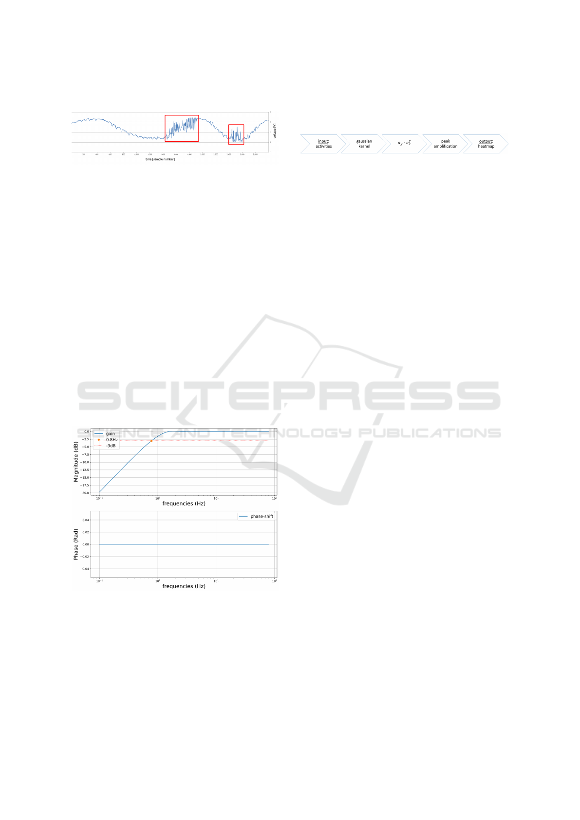
tioned aliasing effects of the ambient 50Hz ﬁeld.

Figure 4: Voltage of a single electrode. Areas marked in red

show walking activities on the electrode.

We use this new signal as a baseline and subtract it

from the original signal. The resulting high pass ﬁlter

is applied for each sensor independently.

Afterwards we pick the sample in the middle of

the ﬁltered window as the new sensor value. We do

that because the FFT is most accurate for the center of

a window and hence the center has the most accurate

baseline.

This step results in a dead-time of the ﬁlter which

is half the size of the window and thus the window

size requires a balance between the frequency resolu-

tion of the FFT and the dead-time of the ﬁlter. Ad-

ditionally, due to the use of the FFT the number of

samples must be a power of two.

Therefore, our ﬁlter has a window size of 64 sam-

ples resulting in a dead-time of 0.64 seconds (32 sam-

ples at a sampling rate of 20 milliseconds). For sim-

plicity, a rectangular window function was used to

clip the window from the signal. The ﬁnal ﬁlter is

characterized by the bode plot in ﬁgure 5.

Figure 5: Bode-plot of the fft-baseline. This plot does not

model the dead-time of the window-function used by the fft.

After removing the baseline, we calculate the ab-

solute value of the ﬁltered sensor measurements and

normalize them. Even though, the maximum of the

sensor values is 4095 since the resolution of the used

ADC is 12bit, the algorithm caps all measured val-

ues to 255 to make better use of the normalized space

between 0 and 1. The cap was applied after baselin-

ing and smoothing through the use of the FFT be-

cause these pre-processing steps are the reason that

high sensor values over 255 were unlikely to occur.

Figure 6: Processing pipeline for the inference of all ampli-

tudes.

Further we established a method to infer a

heatmap from the pre-processed sensor values which

can be seen in ﬁgure 6. First, we emphasize the in-

ﬂuence of close sensors to their positions by using a

discrete normal distribution for the weights of the sen-

sors. The mean represents the position for each sensor

whereas the variance indicates the level of inﬂuence

between neighboring sensors. We optimized the vari-

ance visually while walking over the smart ﬂoor. By

removing the values close to zero this resulted in the

following two gaussian kernels k

, k

for the x and the

y direction.

= (0.001, 0.140, 0.718, 0.140, 0.001)

= (0.016, 0.221, 0.527, 0.221, 0.016)

These values are well suited for visualization of the

heatmap since they are optimized towards a trade-off

between sharpness and blurriness in regions of active

sensors. We then apply the kernels with a zero-padded

convolution to the 12 sensors in x and the 18 sensors

in y direction which gives us the horizontal a

∈ R

and the vertical sensor activities a

∈R

for each po-

sition as a vector.

By calculating the dot product of those vectors

·a

= H ∈R

18×12

we receive a matrix of the corre-

lating sensor activities. This matrix gives us the infor-

mation how active a position or region on the smart

ﬂoor is and hence we call it the heatmap H. Because

of the use of the gaussian kernels which was described

beforehand, a visualization of this matrix with differ-

ent colors will already result in an image with smooth

color gradients.

To further emphasize the remaining peaks in the

heatmap and to make them more persistent in time

we use exponential moving average (Hyndman et al.,

2008) on each element a

t+1

of the heatmap with re-

spect to the previous activity a

of the last time frame.

ˆa

t+1

= αa

+ (1 −α) ˆa

If the new activity is higher than the old activity we

apply a high smoothing factor of α = 80% otherwise

a low smoothing factor of α = 1.5% is applied. This

results in the ﬁnal heatmap

H for each time frame.

The last step is to extract the position of the person

from the heatmap. First, we apply an average ﬁlter on

the heatmap

H so that close local maxima can merge

Neural Networks for Indoor Localization based on Electric Field Sensing

together which happens due to the fact that a walk-

ing person creates two active regions because they

have two feet. Secondly, we search the maximum of

the heatmap matrix because in this evaluation, we are

only interested in a single user scenario and therefore

do not need to cluster regions of activity. The coor-

dinates of the maximum represent the position of the

person.

2.2 ANN Approach

In contrast to the analytic approach we shall now

present a data driven approach with artiﬁcial neural

networks (ANN). Therefore, the next sections will

ﬁrst explain the process of the data acquisition since

the underlying data represent a crucial part of every

machine learning driven approach. Then, we will

present the different model architectures that were de-

signed for the localization of a person moving on the

smart ﬂoor.

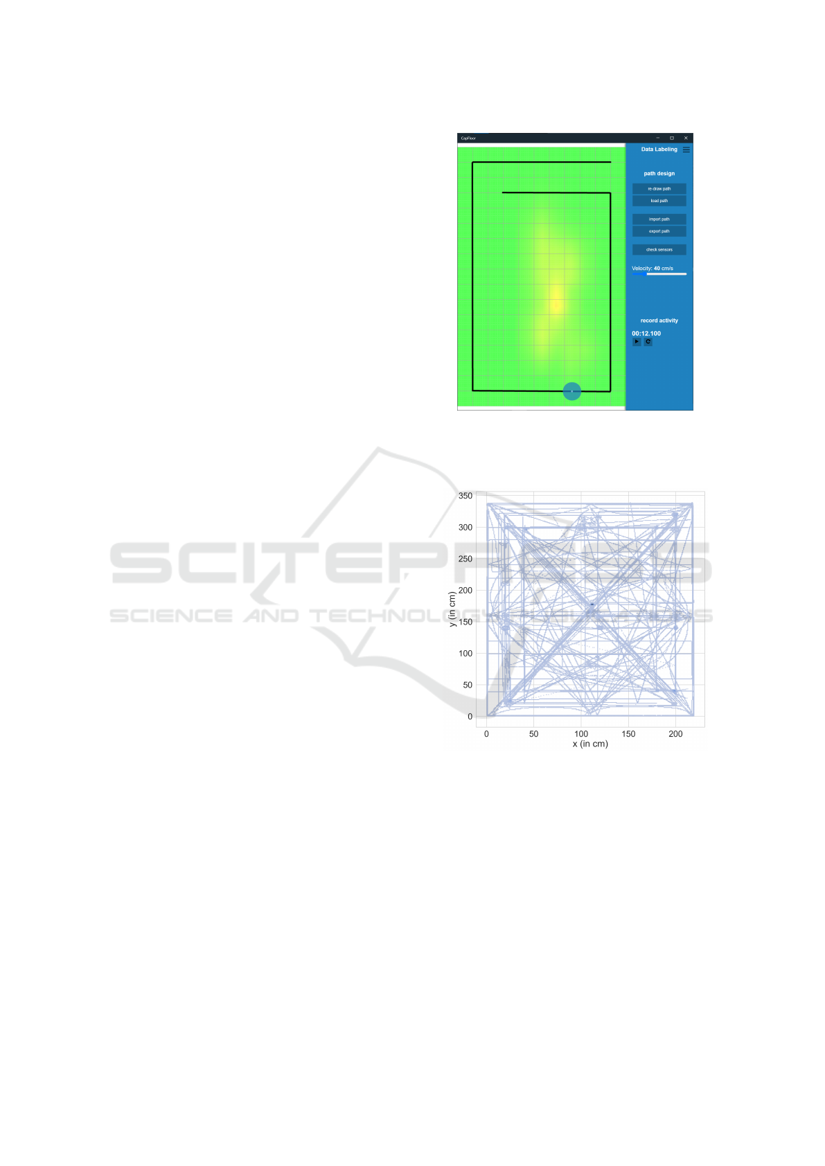
2.2.1 Data Labeling

Our data labeling tool combines the sensor values

with a timestamp and the normalized position which

is the position on the smart ﬂoor with values between

zero and one for both axis. For this purpose, users can

draw a path (polyline) on the virtual depicted ﬂoor to

walk on and set their walking velocity in the GUI to

increase variability of the data (see ﬁgure 7). When

a user starts recording, a circle indicates the position

of the current label and thus the position where the

person should be standing. The circle will then move

along the previously drawn path, which the user has to

follow to generate the corresponding sensor data. All

labels are stored as a normalized position p ∈ [0, 1]

on the smart ﬂoor.

Figure 8 illustrates all paths that were recorded,

added in a single image, using absolute coordinates.

Note that this ﬁgure only contains pathways as cre-

ated by the ground truth data. The data shows that all

regions of the smart ﬂoor were covered.

2.2.2 Model Architecture

We will ﬁrst discuss the input since it is the most rele-

vant factor for the architecture design. The input uses

the raw sensor values without any pre-processing to

avoid loosing information in the process and keeping

the choice of relevant patterns to the training process.

Moreover, changes in the pre-processing step would

require to retrain the models since the patterns in the

input change. However, one should note that this im-

plies an additional challenge to the ANN because it

Figure 7: Data labeling tool GUI to produce a dataset of

labeled sensor activities with the true position of a person.

The person needs to walk on a path while recording (ﬂoor

heatmap on the left).

Figure 8: Ground truth data of all recorded pathways.

has a more complex task at hand, which requires more

training.

The ﬁrst type of input data is the concatenation of

the latest sensor values in the x and y direction. This

results in a vector s ∈ R

with the number of sensors

n = 30.

The second type of input data incorporates the his-

tory of the sensor values to include additional infor-

mation and improve the stability of the predictions

over time. To do that, the concatenated sensor val-

ues s can be stacked together to a matrix (s

, ..., s

) =

I ∈ R

n×t

for t time frames. I is labeled with the latest

label of s

to avoid learning a dead time in the model.

DeLTA 2022 - 3rd International Conference on Deep Learning Theory and Applications

In all architectures the output layer is a fully-

connected (FC) layer with two output units followed

by a sigmoid activation function. The two units be-

tween zero and one correspond to the normalized co-

ordinates of a person on the smart ﬂoor. The upper left

corner corresponds to the (0,0) coordinates and the

lower right corner corresponds to the position (1,1).

Next, a clariﬁcation of the tested architectures will

be listed to show their differences in structure and

complexity.

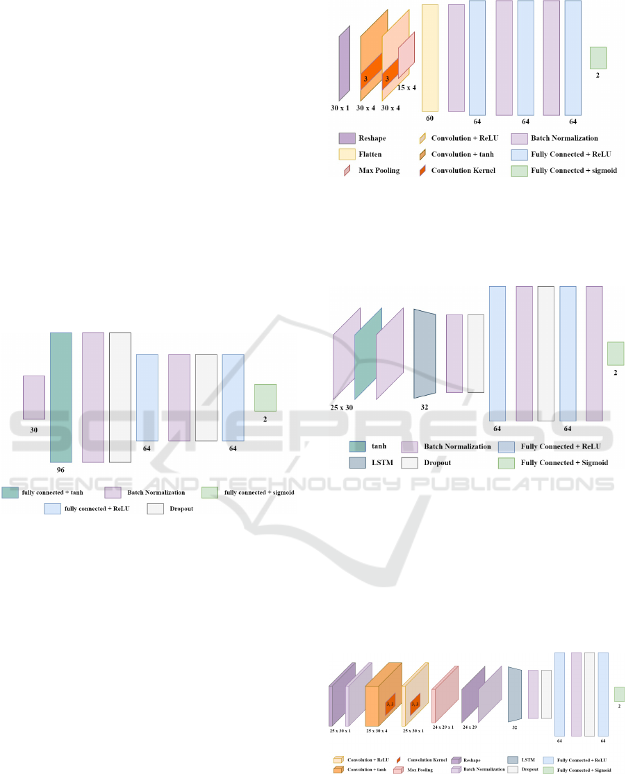
The Dense architecture (ﬁgure 9) has 13,854

trainable parameters and is mainly composed of three

FC layers plus the output layer. It uses the latest state

of the sensors s as input.

Due to the lack of pre-processing, the network

uses a batch normalization (BN) layer before each FC

layer and tanh as activation function after the ﬁrst FC

layer. After the other FC layers the ReLU activation

functions (Rectiﬁed Linear Unit) is used, except for

the output layer.

Figure 9: Structure visualization of the Dense architecture.

The CNN1D architecture (ﬁgure 10) uses the s

vector as input and is similar to the Dense architecture

but applies additional pre-processing with use of local

feature extraction in the ﬁrst layers. Speciﬁcally, it

uses 1D convolutional layers (Conv1D), BN and pool-

ing layers to enable the extraction of local features

from neighboring sensors. The ﬁrst Conv1D layer is

followed by a tanh activation function to reduce the

inﬂuence of peaks in the data which can occur due to

wrong sensor measurements or errors emerging from

the data transmission on the used bus system. All

other activation functions continue with ReLU func-

tions. It has 12,800 trainable parameters.

The RNN architecture (ﬁgure 11) introduces the

use of time information and uses the time matrix input

I as described earlier. The architecture begins with a

BN layer followed by a tanh activation function on

the input to reduce the inﬂuence of peaks in the data.

It proceeds with a BN and a LSTM layer (long short

term memory) (Hochreiter and Schmidhuber, 1997)

Figure 10: Structure visualization of the CNN1D architec-

ture.

to process the time information. These are then fol-

lowed by two blocks of BN and FC layers plus the

output layer. It has 14,906 trainable parameters.

Figure 11: Structure visualization of the RNN architecture.

The CRNN architecture (ﬁgure 12) is similarly

motivated as the CNN1D and applies further pre-

processing to the RNN. To achieve this, it consists of

one Conv2D layer with tanh and one Conv2D layer

with ReLU activation function followed by BN and a

max-pooling layer. This is proceeded by a block of

BN and LSTM layers for time processing, a block of

BN and FC layers and the output layer. It has 10,507

trainable parameters.

Figure 12: Structure visualization of the CRNN architec-

ture.

The TCNN architecture (ﬁgure 13) is a CNN ar-

chitecture used on the time input matrix I. It consists

of multiple blocks of Conv2D, BN and pooling lay-

Neural Networks for Indoor Localization based on Electric Field Sensing

ers motivated by the VGGNet model (Simonyan and

Zisserman, 2014). This enables the extraction of lo-

cal features from neighboring sensors and close time

frames. The convolutional blocks are followed by two

FC layers plus the output layer. It has 14,948 trainable

parameters.

Figure 13: Structure visualization of the TCNN architec-

ture.

3 RESULTS

In this section, we will present out ﬁndings of the ac-

curacy for the different neural networks as well as the

results of the formerly discussed analytical approach.

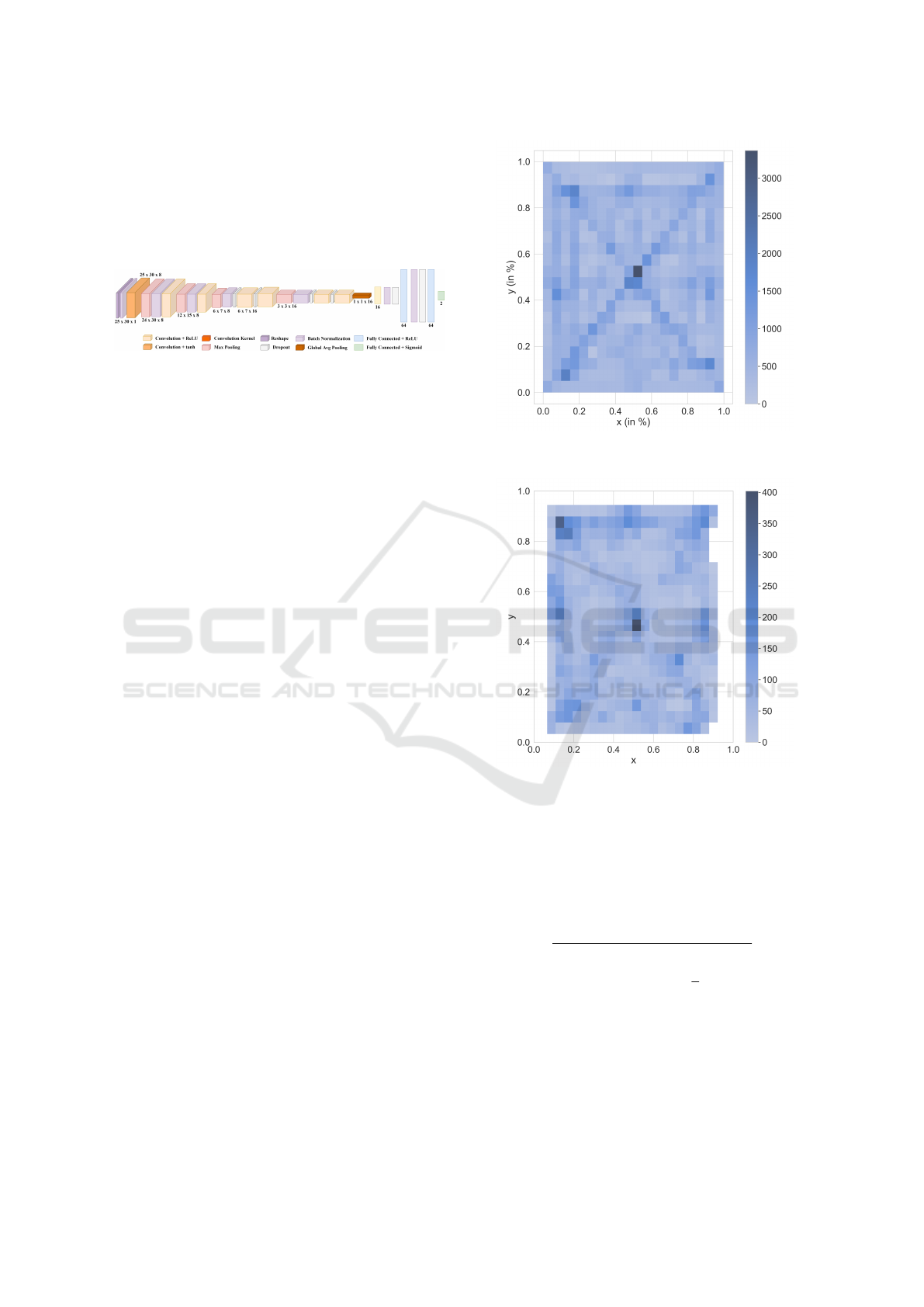
3.1 Dataset

For training the different neural networks, we col-

lected 31 different path patterns from 4 test persons,

resulting in 258 data sheets. Combined to datasets

gives a total record duration of 4400 seconds of

persons walking over the smart ﬂoor equivalent to

220’023 samples of sensor-frames. A sensor-frame

consists of the aggregation of all sensors values within

a single time frame. A single sensor operates at a sam-

ple rate of 50 samples per second. These samples are

fairly distributed over the smart ﬂoor with a peak in

the center as you can see in ﬁgure 14. The dataset is

split into train (89%) and test (11%) datasets. The test

dataset is used to evaluate the models. This can also

be seen by comparing Figure 14 and Figure 15. While

the number of predictions in a single spot in Figure

14 sum up to over 3000 labeled positions per cluster,

there are much less predictions per cluster in Figure

15 just because of the different sizes of datasets.

As shown in Figure 16, using this test- and train-

ing dataset, all models will converge after approx-

imately 50 steps of training. The euclidean dis-

tance between the ground truth position of the user

and the calculated position from the respective net-

work is used to express the error. The training pro-

cess was terminated after 100 steps, since the conver-

gence nearly stopped afterwards for all models. The

Dense architecture showed signs of over-ﬁtting after

80 training iterations. Figure 16 also hints that the

TCNN architecture converges faster than other mod-

els with a lower overall error.

Figure 14: Histogram of the labeled positions on the smart

ﬂoor showing how even the samples are distributed.

Figure 15: Histogram of all predictions of the validation set

from the TCNN model.

3.2 Model Performance

The evaulation of our methods is based on the eu-

clidean error. It is deﬁned as the euclidean distance

between the model prediction and the true position of

the person.

pred

−x

true

)

+ (y

pred

−y

true

)

This gives us a range from 0 to

√

2 since x and y are

normalized. One should note that the percent values

are simply scaled by 100 and therefore range from 0

to 141.42%.

The model performances differ in the x and y di-

rection due to the fact that our smart ﬂoor setup is

220cm wide and 340cm long with evenly spaced sen-

sors at a distance of 20cm in both directions resulting

DeLTA 2022 - 3rd International Conference on Deep Learning Theory and Applications

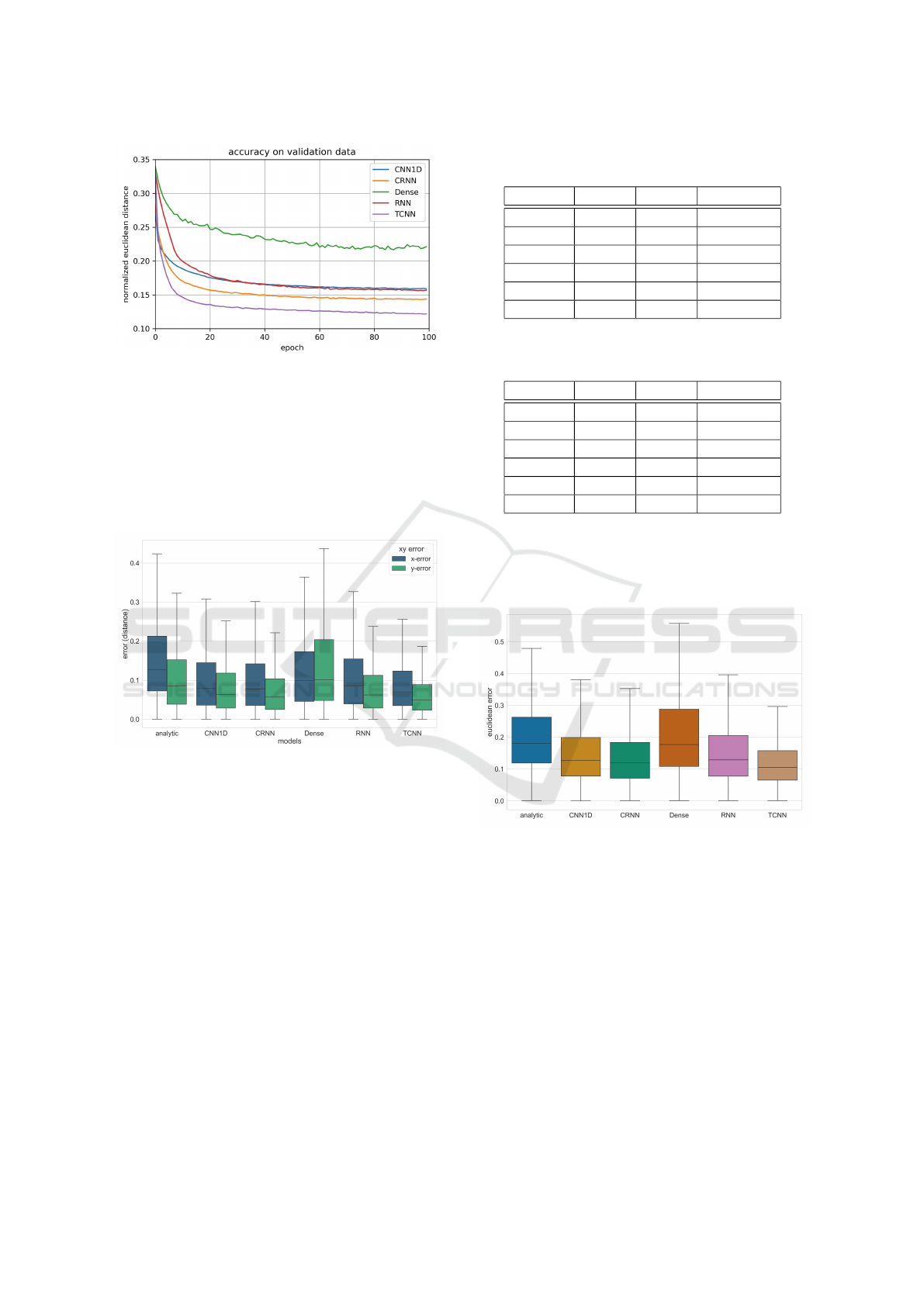
Figure 16: Comparison of the model performance on the

validation data during training.

in more data on the y axis. This difference of the nor-

malized distance can be seen in ﬁgure 17. However,

the scaled error to the true size of the smart ﬂoor re-

sults in a higher accuracy in the x direction due to the

higher scaling factor in the y-direction. The tables 1

for the normalized results and 2 for the results in cen-

timeters show these differences.

Figure 17: Visualization of the error in the x and y direction.

We can see that the convolutional pre-processsing

increases the performance for both CNN1D and

CRNN compared to the non-convolutional architec-

tures Dense and RNN. The performances are listed in

the following table 1 and visualized in ﬁgure 18.

After all, the TCNN was the best performing ar-

chitecture with the best model having a average accu-

racy of 12.8% and shows to have a good distribution

of predictions on the smart ﬂoor with no signiﬁcant

bias as shown in ﬁgure 15. Another good indicator

of the model performances is that the overall shape of

Figure 14 can be recognized in 15.

Since the use of local feature extraction has shown

to be beneﬁcial it is reasonable that the TCNN model

performed best, as it utilizes multiple layers for this

purpose. Moreover, the RNN did not perform as well

as the TCNN architecture which might be confusing

at ﬁrst because it is a well established architecture

for time series data. This is because the LSTM uses

Table 1: The average errors of the models on the normalized

smart ﬂoor. All values in [%].

model x-error y-error eucl.-error

TCNN 9.17 7.03 12.83

CRNN 10.24 8.35 14.77

CNN1D 10.46 9.46 15.91

RNN 11.31 9.07 16.17

analytic 15.63 11.47 21.24

Dense 12.50 15.02 21.72

Table 2: The average errors of the models on the real scale

of the smart ﬂoor. All values in [cm].

model x-error y-error eucl.-error

TCNN 20.2 23.9 34.8

CRNN 22.5 28.4 40.5

CNN1D 23.0 32.2 44.3

RNN 24.9 30.8 44.2

analytic 34.4 39.0 57.3

Dense 27.5 51.1 63.2

global feature extraction for the time series. As previ-

ously inferred by the results of the other architectures,

this lacks the use of local feature extraction of neigh-

boring sensors and therefore tends to over-ﬁt.

Figure 18: The euclidean-error of the normalized smart

ﬂoor. The box size represents the interquartile range.

4 DISCUSSION

The artiﬁcial neural networks provided a large im-

provement compared to the analytic approach. But

even if models perform seemingly the same com-

pared by error rate and convergent rate, such as the

RNN and the CNN1D architectures, their behavior

while displaying the position of a user in a live plot

can still differ signiﬁcantly. While the RNN shows

much smoother transitions of the displayed position

of the user roaming over the smart ﬂoor, the posi-

tion displayed by the CNN1D has a strong jitter ef-

Neural Networks for Indoor Localization based on Electric Field Sensing

fect. The displayed position seemingly jumps around

the real user position in an uncontrolled manner. This

is because the RNN uses the information of multiple

time steps while the CNN1D only uses the latest time

frame of the sensor values. That is why, in the case of

these two architectures, the RNN network should be

preferred over the CNN1D.

Overall, using neural networks for this kind of

problem is a better approach than a purely analytical

one, since our problem can be modeled as a function

which maps values from the sensor measurements to

a person position. That is why this problem is well

suited for supervised learning techniques like neural

networks. Since we were able to label a good amount

of samples the NN approaches had much more op-

timization steps than the manually adjusted analytic

approach.

However, the dataset is still relatively small and

should by the focus of further studies to improve the

precision even further. As, for example, shown by

Chung et al. in their publication ”VoxCeleb2: Deep

Speaker Recognition”(Chung et al., 2018), a larger

dataset for training can decrease the error of a network

signiﬁcantly. In their paper, the authors train a neural

network to recognize the voice of different celebrities.

They also use different datasets with different sizes

to train the same model. The result is a signiﬁcantly

lower error rate by using the larger dataset.

Another important point of the data acquisition is

the labeling method. As already stated in section 2, in

order to record training data, a test person has to fol-

low an indicated position on a screen while walking

on a predeﬁned pattern. The GUI provides a method

for fast and easy labeling and can be used by users

which are unfamiliar with the system. A down side

was the accuracy of the labels because users could

not determine the exact position of themselves on the

smart ﬂoor. Hence, the persons had to orientate them-

selves by estimating the position of the shown set-

point of the software. This is possible since the used

localization system has a relatively small size, but not

optimal in terms of repeatability.

The vision for the presented system is to install

a smart ﬂoor in a large amount of nursing homes

and hospitals. At the moment, this would require

a completely new dataset for each new smart ﬂoor

and the computationally intense training of a model.

Both of these tasks, especially the collection of a

dataset that also includes the necessary test data, are

very time consuming tasks and have to be realized

even for smart ﬂoors that are covering a small spa-

cial area. Therefore, further studies should investi-

gate size-invariant architectures similar to the TCNN

and one shot learning models to scale to those appli-

cations. However, the use of convolutional neural net-

works alone which can make the model size-invariant

will not accomplish this goal since the length of the

sensor electrodes changes in nearly every environ-

ment. This also changes the magnitude of the sen-

sor measurements, resulting again in the need of a

new data collection and training. Even a normaliza-

tion of the measured data is limited in its use because

the changes of the length of the wires used as elec-

trodes when scaling up a smart ﬂoor will in practice

never keep the ratio between the length of wires in

x-direction and y-direction. The analytical approach

struggles with the same problem. Fortunately as for

the analytical approach, this problem can be reduced

with a calibration routine which identiﬁes the minimal

and maximal sensor values for each sensor by walking

over them once. As shown, this approach is signiﬁ-

cantly less accurate than the use of neural networks.

This is why one of the most important topics for fu-

ture work will tackle the problem of size-invariant lo-

calization based on neural network architectures.

5 SUMMARY

This paper has presented an analytical approach for

the localization of a single person on the smart ﬂoor

as well as multiple neural networks to accomplish this

task. Moreover, we presented a tool for data acquisi-

tion and labeling and the resulting dataset of 220’023

samples.

Our Data showed that the TCNN architecture is

the method with the highest position accuracy com-

pared to the Dense, CNN1D, RNN and CRNN archi-

tecture. With an euclidean error of 34.8cm on average

which is an improvement of 22.5cm to the previously

used analytic method with an error of 57.3cm on av-

erage, the TCNN reduced the overall error by 40%.

We have also shown that the use of convolutions as

ﬁrst layers for local feature extraction in the time do-

main and with neighboring sensors of the smart ﬂoor

resulted in signiﬁcant better performance.

Overall, the data driven machine learning ap-

proach seems promising even though it suffers from

the missing scalability to multiple smart ﬂoors with

different sensor layouts.

REFERENCES

Chung, J. S., Nagrani, A., and Zisserman, A. (2018). Vox-

celeb2: Deep speaker recognition. Interspeech 2018.

Faulkner, N., Parr, B., Alam, F., Legg, M., and Demi-

denko, S. (2020). Caploc: Capacitive sensing ﬂoor

DeLTA 2022 - 3rd International Conference on Deep Learning Theory and Applications

for device-free localization and fall detection. IEEE

Access, 8:187353–187364.

Frank, S. and Kuijper, A. (2020). Privacy by design: Analy-

sis of capacitive proximity sensing as system of choice

for driver vehicle interfaces. In Stephanidis, C., Duffy,

V. G., Streitz, N., Konomi, S., and Kr

omker, H., edi-

tors, HCI International 2020 – Late Breaking Papers:

Digital Human Modeling and Ergonomics, Mobility

and Intelligent Environments, pages 51–66, Cham.

Springer International Publishing.

Fu, B., Damer, N., Kirchbuchner, F., and Kuijper, A.

(2020a). Sensing technology for human activity

recognition: A comprehensive survey. IEEE Access,

8:83791–83820.

Fu, B., Kirchbuchner, F., and Kuijper, A. (2020b). Data

augmentation for time series: Traditional vs genera-

tive models on capacitive proximity time series. In

Proceedings of the 13th ACM International Confer-

ence on PErvasive Technologies Related to Assistive

Environments, PETRA ’20, New York, NY, USA. As-

sociation for Computing Machinery.

Hochreiter, S. and Schmidhuber, J. (1997). Long short-term

memory. Neural Computation, 9(8):1735–1780.

Hyndman, R., Koehler, A. B., Ord, J. K., and Snyder, R. D.

(2008). Forecasting with exponential smoothing: the

state space approach. Springer Science & Business

Media.

Kirchbuchner, F., Grosse-Puppendahl, T., Hastall, M. R.,

Distler, M., and Kuijper, A. (2015). Ambient intelli-

gence from senior citizens’ perspectives: Understand-

ing privacy concerns, technology acceptance, and ex-

pectations. In De Ruyter, B., Kameas, A., Chatzimi-

sios, P., and Mavrommati, I., editors, Ambient Intel-

ligence, pages 48–59, Cham. Springer International

Publishing.

Nam, H., Seol, K.-H., Lee, J., Cho, H., and Jung, S. W.

(2021). Review of capacitive touchscreen technolo-

gies: Overview, research trends, and machine learning

approaches. Sensors, 21(14).

Obeidat, H., Shuaieb, W., Obeidat, O., and Abd-Alhameed,

R. (2021). A review of indoor localization techniques

and wireless technologies. Wireless Personal Commu-

nications, 119(1):289–327.

Roy, P. and Chowdhury, C. (2021). A survey of machine

learning techniques for indoor localization and navi-

gation systems. Journal of Intelligent & Robotic Sys-

tems, 101(3):63.

Simonyan, K. and Zisserman, A. (2014). Very deep con-

volutional networks for large-scale image recognition.

arXiv preprint arXiv:1409.1556.

Neural Networks for Indoor Localization based on Electric Field Sensing