An Ensemble-based Dimensionality Reduction for Service Monitoring

Time-series

Farzana Anowar

1,2 a

, Samira Sadaoui

1 b

and Hardik Dalal

University of Regina, Regina, Canada

Ericsson Canada Inc., Montreal, Canada

Keywords:

Service Monitoring, High-dimensional Time-series, Dimensionality Reduction, Incremental Dimensionality

Reduction, Clustering Quality, Data Reconstruction.

Abstract:

Our work introduces an ensemble-based dimensionality reduction approach to efﬁciently address the high

dimensionality of an industrial unlabeled time-series dataset, intending to produce robust data labels. The en-

semble comprises a self-supervised learning method to improve data quality, an unsupervised dimensionality

reduction to lower the ample feature space, and a chunk-based incremental dimensionality reduction to further

increase conﬁdence in data labels. Since the time-series dataset is massive, we divide it into several chunks

and evaluate each chunk’s quality using time-series clustering method and metrics. The experiments reveal

that clustering performances increased signiﬁcantly for all the chunks after performing the ensemble approach.

1 INTRODUCTION

In industry, an incredible amount of data is produced

daily, and in many applications, data need to be pro-

cessed and analyzed in real-time. Even though ma-

chine learning algorithms can handle a vast quan-

tity of data, their performances worsen as the fea-

ture space becomes larger (Van Der Maaten et al.,

2009), (Spruyt, 2014). The predictive models become

more complex as the dataset’s size and dimension-

ality increase (Verleysen and Franc¸ois, 2005), (Jin-

dal and Kumar, 2017). Decision models trained on

a large feature space become reliant on the data and

may over-ﬁt (Hawkins, 2004), (Anowar et al., 2021).

Additionally, the models’ accuracy declines due to

the presence of similar or irrelevant features (Jindal

and Kumar, 2017). This problems get worse when

high-dimensional time-series data is produced. Reg-

ular machine learning algorithms cannot handle the

continuous time-series data (Losing et al., 2018). Our

study emphasizes an industrial application on service

availability, which allows users to check what our

servers are up to. Hence, data are crawled continu-

ously or periodically with higher data dimensionality

for monitoring services’ availability. A robust Service

Monitoring dataset was developed in (Anowar et al.,

https://orcid.org/0000-0002-1535-7323

https://orcid.org/0000-0002-9887-1570

2022), which is temporal, unlabeled, and highly di-

mensional.

Furthermore, many machine learning methods fail

to perform efﬁciently in real-world scenarios because

of having inadequate target labels. Hence, it is crucial

achieving the highest conﬁdence for the class labels.

For this purpose, we introduce an ensemble-based di-

mensionality reduction approach to efﬁciently pro-

cess an industrial use case’s high dimensional, non-

linear, and unlabeled time-series dataset with two ob-

jectives: 1) to better the data quality and 2) to produce

highly conﬁdent data labels. For the experimental

purpose, we have taken the new Service Monitoring

dataset from (Anowar et al., 2022), and we partition

the dataset into six week-by-week chunks.

The ensemble approach combines four methods

to handle this particular time-series dataset: a self-

supervised learning method, an unsupervised dimen-

sionality reduction, an incremental dimensionality re-

duction, and a time-series clustering. As a self-

supervised method, we adopt Autoencoder to recon-

struct the chunks in better data spaces by ignoring dis-

turbances, such as noisy and insigniﬁcant data. Sub-

sequently, we utilize the Kernel PCA (KPCA), an un-

supervised dimensionality reduction method, to re-

duce the ample feature spaces of the reconstructed

chunks into much shorter representations. Fewer di-

mensions mean less computation, faster training, eas-

ier data visualization, and less storage. The ulti-

Anowar, F., Sadaoui, S. and Dalal, H.

An Ensemble-based Dimensionality Reduction for Ser vice Monitoring Time-series.

DOI: 10.5220/0011273700003277

In Proceedings of the 3rd International Conference on Deep Learning Theory and Applications (DeLTA 2022), pages 117-124

ISBN: 978-989-758-584-5; ISSN: 2184-9277

117

mate goal of this research is to obtain the highest

level of conﬁdence in the data labels for the Service

Monitoring dataset. For this purpose, we employ a

chunk-based incremental KPCA, an unsupervised in-

cremental dimensionality reduction method proposed

in (Tokumoto and Ozawa, 2011). We apply the incre-

mental learning method to each of the previously re-

duced chunks to improve the clustering performance

so that the cluster’s labels are accurate. We utilize the

cluster’s labels as the target data labels. We do not

consider the incremental KPCA to reduce the dimen-

sionality of the chunks; instead, we improve the data

quality.

To the best of our knowledge, there are minimal

incremental dimensionality reduction methods avail-

able for the supervised setting in the literature. This

limitation is even worse when dealing with non-linear

and unlabeled data (i.e., unsupervised). The chunk-

based incremental KPCA proposed in (Tokumoto and

Ozawa, 2011) is the only incremental dimensionality

reduction method that is chunk-based as opposed to

the instance-based incremental dimensionality reduc-

tion methods, and this is why we choose it.

Experimental results disclose that we obtain high

clustering performances with the ensemble-based

chunks. The latter outperforms the performances of

the initial chunks in all cases. Better clustering per-

formances ensure that the clusters are of better quality

where intra-cluster distances are maximized and inter-

cluster distances are minimized. In addition to that,

we will attain higher conﬁdence in the target labels

for the further decision-making task for the industrial

partner.

We organize our paper as follows. Section 2 dis-

cusses recent literature on the efﬁcacy of Incremen-

tal KPCA. Section 3 summarizes the characteristics

of the Service Monitoring dataset and then divides

it into multiple weekly chunks. Section 4 details

the proposed ensemble-based dimensionality reduc-

tion framework to produce accurate data labels. Sec-

tion 5 presents the experiments to assess the effec-

tiveness of the ensemble method in terms of clusters’

quality. Section 6 concludes our study and highlights

some future works.

2 RELATED WORKS

The very few incremental, unsupervised dimension-

ality reduction techniques have been deﬁned in (Kim

et al., 2005), (Chin and Suter, 2007), (Takeuchi et al.,

2007), (Tokumoto and Ozawa, 2011). However, most

of them are instance-based where incoming data are

processed instance by instance. One of the very

ﬁrst Incremental KPCA was proposed in (Kim et al.,

2005), which is based on the ‘Generalized Hebbian

Algorithm’ presented as an online algorithm for linear

PCA in (Sanger, 1989), (Oja, 1992). The hybrid algo-

rithm iteratively estimates the kernel principal com-

ponents using only a linear order memory complexity,

which makes it suitable for large datasets. However,

until an adequate accuracy is achieved, this Incremen-

tal KPCA necessitates a high number of learning iter-

ations.

(Chin and Suter, 2007) developed an incremental

KPCA that is based on the incremental linear PCA

introduced in (Lim et al., 2004). The Eigen-feature

space is incrementally updated instance by instance

in this proposed Incremental KPCA by performing

Singular Value Decomposition on the incoming train-

ing data. However, the Eigen-space model is updated

without learning all of the training data repeatedly,

this approach can be called a one-pass incremental

learning algorithm. Furthermore, higher memory and

computation costs are required to construct a reduced

dataset. The time and memory complexities are O(n

)

and O(n

), respectively for this algorithm.

The study (Takeuchi et al., 2007) proposed an in-

cremental KPCA where an eigen-feature space is rep-

resented by a combination of linearly independent

data, allowing it to learn from new data incremen-

tally without having to remember previous training

data. However, an open problem remains in this pro-

posed algorithm, is that an eigen-feature space should

be updated by solving an eigen value problem only

when new training data is received, which means that

eigen-value decomposition should perform for each

data in the chunk individually to update the eigen-

feature space, which leads to higher time and mem-

ory complexity, and it can only update eigen-vectors

quickly with a small set of linearly independent data

(lower dimensionality). Additionally, if the chunk

size is larger, real-time online feature extraction may

be impossible.

Later, the research (Tokumoto and Ozawa, 2011)

proposed a chunk-based incremental KPCA that con-

ducts the Eigen-feature space learning by only exe-

cuting the Eigen value decomposition once for each

chunk of incoming training data. The cumulative pro-

portion is used to choose linearly independent data

whenever a new chunk of training data becomes avail-

able. Then, the Eigen-space augmentation is per-

formed by measuring the coefﬁcients for the chosen

linearly independent data, and the Eigen-feature space

is rotated based on the rotation matrix generated by

solving a kernel Eigen value problem. So far, this

proposed chunk-based algorithm is the most efﬁcient

Incremental KPCA.

DeLTA 2022 - 3rd International Conference on Deep Learning Theory and Applications

118

The authors in (Joseph et al., 2016) proposed an

incremental KPCA by extending the algorithm de-

ﬁned in (Takeuchi et al., 2007) to make it work for

the chunk setting. In this incremental KPCA, ﬁrst,

a chunk of data is split into several smaller chunks

since author considered that retaining a suitable size

of data chunk is vital for fast learning. Then, from

the divided data chunks, only important features are

selected using regular KPCA, because not all data in

a chunk are valuable for learning. In the proposed in-

cremental KPCA, an Eigen-feature space is spanned

by Eigen vectors that are presented by a linear com-

bination of independent data. Later, a rotation matrix

to update the Eigen vectors and an Eigen value matrix

is attained by solving an Eigen value decomposition

problem only once for given data chunk. However, re-

ducing a chunk twice and keeping only few data from

a chunk is not practical always when processing real-

world dataset like time-series.

3 AN INDUSTRIAL TIME-SERIES

DATASET

Our past study (Anowar et al., 2022) developed a

Service Monitoring time-series, a new highly di-

mensional and unlabeled dataset derived from an in-

dustrial application, so developers can monitor ser-

vice availability, react to changes in service-wide

performance, and optimize service allocation. The

dataset was constructed from 48 sub-servers that used

Prometheus to collect data every 15 seconds for var-

ious services for over six weeks in the year 2020.

The chunks, containing information over six weeks

(39 days), come in different sizes and feature sets. A

dataset sample denotes the service’s availability, UP

or DOWN, for a given point of time. For example,

one instance may show that the service is up at 12.01

a.m., while another instance may suggest that the ser-

vice is down at 5.00 a.m. The Service Monitoring

data can be of two types: 1) Counter type indicating

a monotonically growing counter whose value can ei-

ther increase or be reset to zero on the restart, and 2)

Gauge type denoting a single numerical value that can

arbitrarily go up and down (Anowar et al., 2022). A

detailed description of this dataset is provided in past

work (Anowar et al., 2022).

The Service Monitoring dataset is large, compris-

ing 53,953 data and 3100 features. Hence, it requires

enormous memory space to be processed, particularly

when performing the KPCA method. The latter ne-

cessitates a sizeable short-term memory to perform

the kernel function and store the large kernel matrix

to project data to higher feature space so that data can

be linearly processed (Goel and Vishwakarma, 2016).

Hence, it is impossible to perform the kernel on the

whole dataset. Therefore, we split the dataset into six

chunks, one chunk for each week. This split enables

processing chunks in an incremental manner.

The ﬁrst chunk possesses 9,099 data, the sixth

chunk has 4,534 data, and the four others have 10,080

data. These chunks have the same size because they

have the same amount of time for seven days, starting

at midnight and ending at 11.59 pm. The data collec-

tion for the ﬁrst day of the ﬁrst week began at 4.21

pm, and the last week has only four days. Table 1

presents the size and dimensionality for each chunk.

Table 1: Size and Dimensionality of Weekly Chunks.

Chunk Size Dimensionality

#1 9,099 3,100

#2 10,080 3,100

#3 10,080 3,100

#4 10,080 3,100

#5 10,080 3,100

#6 4,534 3,100

4 ENSEMBLE-BASED

DIMENSIONALITY

REDUCTION

When data come with high dimensionality, the train-

ing process for machine learning algorithms becomes

difﬁcult, resulting in over-ﬁtting the decision models

and lowering their performances (Jindal and Kumar,

2017). These problems are even worse when process-

ing complex data like time series. To this end, we

propose an ensemble-based dimensionality reduction

approach to manage unlabeled, non-linear, and high-

dimensional time-series chunks, intending to improve

each chunk’s quality and increase its labeling conﬁ-

dence.

We ﬁrst utilize a self-supervised learning method

on each time-series chunk to reconstruct its data and

improve its quality. Then, we adopt an unsupervised

dimensionality reduction technique to efﬁciently re-

duce the ample feature space. The reduced chunk is

then passed to an incremental, unsupervised dimen-

sionality reduction method not to lower the dimen-

sionality but to improve the data quality further and

increase the chunk labels’ conﬁdence. Lastly, we as-

sess the quality of the ﬁnal chunks by checking their

clustering performances to decide on the cluster la-

bels and show the necessity of our approach. The fol-

lowing section describes each phase of the ensemble-

based dimensionality reduction approach.

An Ensemble-based Dimensionality Reduction for Service Monitoring Time-series

119

4.1 Data Reconstruction of Each Chunk

We adopt a deep autoencoder model (named DAE)

as a pre-processing phase to increase data quality

by removing noisy data without changing the feature

space. Besides, DAE can process non-linear data,

like ours, efﬁciently by adopting non-linear activa-

tion functions in hidden and output layers (Almotiri

et al., 2017). DAE consists of two parts: 1) the en-

coder compresses the input data to a smaller encoding

with a latent space, and 2) the decoder reconstructs

the compressed data as closely as possible (Wang

et al., 2016). DAE learns from data when back-

propagating through the neural network and exclud-

ing irrelevant discrepancies during encoding, result-

ing in an accurately reconstructed dataset (Lawton,

2020). The DAE aims to minimize the reconstruc-

tion loss; the smaller the loss, the reconstructed data is

more likely to be the original data (Wang et al., 2016).

We ﬁrst train DAE with the whole time-series dataset

to tune the hyper-parameters (hidden layers, weight

optimizer, loss function, batch size, epoch number,

and stopping criterion) and also determine the optimal

architecture. This DEA conﬁguration will be utilized

for each weekly chunk.

4.2 Dimensionality Reduction of Each

Chunk

We make use of the popular feature extraction tech-

nique KPCA to manage each available chunk. The

KPCA method uses the “kernel trick” to project data

into a higher feature space so that data can be linearly

separable (Hoffmann, 2007). We employ RBF as the

kernel function for KPCA to better handle the non-

linearity of data. PCA uses the Eigen decomposition

to produce the Eigen vectors and values (Fan et al.,

2014). The Eigen vectors represent the new obtained

features called Principal Components (PCs).

Before applying KPCA, we search for the best

number of PCs by maximizing the “Total Explained

Variance Ratio” metric (TEVR) to ensure no signiﬁ-

cant lose of information after reconstructing a chunk.

TEVR accumulates the explained variances of all the

PCs. The explained variance of a PC represents

the overall information contained by the PC (Kumar,

2020).

4.3 Incremental Dimensionality

Reduction of Each Chunk

Our objective is to perform the incremental KPCA on

each chunk to improve the clustering performances

and achieve the most conﬁdent cluster labels. We

adopt the chunk-based incremental KPCA algorithm

introduced in (Tokumoto and Ozawa, 2011) and dis-

cussed in Section 2 (related work). This study

(Tokumoto and Ozawa, 2011) provided only the the-

oretical framework. Another work (Hallgren and

Northrop, 2018) implemented this sophisticated al-

gorithm, which is capable of handling the training

chunks sequentially.

No direct library or package is available for incre-

mental KPCA in Python, Matlab, or R programming

languages. To use the incremental KPCA in Jupyter

Notebook, we ﬁrst clone a Git repository from Github

where the implementation of the chunk-based incre-

mental KPCA (Hallgren and Northrop, 2018) was

provided. For using this Git repository efﬁciently,

Python 3.6 or higher versions, Numpy, and Scipy

must be installed. The Git module must be placed in

the same folder as the Python script to invoke the in-

cremental KPCA algorithm. Moreover, the input data

must be passed as an array for this implementation.

Additionally, to extract the desired principal compo-

nents, we have to conduct the dot product of the input

data matrix with the updated Eigen vectors returned

from the incremental KPCA program each time sep-

arately for all the chunks. Moreover, unlike conven-

tional KPCA implementations, this method returns all

the Eigen vectors (PCs) in decreasing order, allowing

users to select the desired PCs (the new features).

4.4 Clustering Evaluation of Each

Chunk

We employ a time-series clustering algorithm for each

ensemble chunk to produce the clusters. We uti-

lize the TS-Kshape method since Service Monitor-

ing dataset is temporal. TS-KShape is a domain-

independent and shape-based time-series clustering

technique (Paparrizos and Gravano, 2015). In each

iteration, TS-Kshape provides the similarity between

two time-series data based on the normalized cross-

correlation to update the cluster assignments (Paparri-

zos and Gravano, 2015). To efﬁciently determine

the centroid of each cluster, TS-Kshape considers the

centroid computation as an optimization problem by

minimizing the sum of the squared distances to all the

other data points from the centroid.

In addition, we consider two as the cluster num-

ber since the Service Monitoring dataset will have

two target labels (Up and Down). We evaluate the

cluster quality of the ensemble chunks using two per-

formance metrics: Davies-Bouldin (named DB) Index

and the Variance Ratio Criterion (named VRC). The

DB Index calculates how similar each cluster is on av-

erage, implying that the intra-cluster distance should

DeLTA 2022 - 3rd International Conference on Deep Learning Theory and Applications

120

be kept to a minimum, and VRC is a criterion that re-

turns the ratio of between-cluster and within-cluster

dispersion (Pedregosa et al., 2011), (Zhang and Li,

2013). The lower, the better for DB Index, and the

higher, the better for VRC (Pedregosa et al., 2011).

5 EXPERIMENTS

5.1 Autoencoder Conﬁguration

To ﬁnd the optimal architecture for DAE, we perform

grid search over multiple hyper-parameters. The best

DEA architecture is composed of six hidden layers

for both encoder and decoder, 1032 for batch size,

Adadelta for the weight optimization, Relu activation

function for all the hidden layers, Sigmoid function

for the output layer, and MSE for the loss function.

For the encoder part, we sequentially provide 3100

(original), 2500, 1650, 1032, 500, 100 and 5 features

using the six hidden layers, and again, we reconstruct

the features from 5, 100, 500, 1032, 1650,2500 and

3100. We utilize ﬁve epochs with no reduction in the

reconstruction loss by 0.0001 as the stopping criterion

for training. We use this optimal DAE conﬁguration

for each incoming chunk individually.

5.2 First Chunk Transformation

We ﬁrst describe the entire transformation process on

chunk #1 to improve the understandability. We train

the optimal DAE conﬁguration on the ﬁrst chunk until

the model’s loss is not converging anymore, intending

to build the best-reconstructed data. After reconstruc-

tion, the chunk will have the same dimensionality as

the initial one but with much better data quality. The

maximum TEVR and optimal PCs for chunk#1 are

0.999920 and 75, respectively. We, therefore, utilize

75 PCs when executing the KPCA algorithm to re-

duce the dimension space and the incremental KPCA

algorithm to produce better quality of data.

We note that the chunks obtained after utilizing

DAE+KPCA are denoted as ”reduced chunks”, and

after applying chunk-based incremental KPCA they

are named ”ensemble chunks”. From Table 2, we ob-

serve that the reduced chunk (DAE+KPCA) outper-

forms the initial chunk with a large margin. The ini-

tial chunk has DB and VRC of 1.552 and 3,455.962,

respectively, whereas the reduced chunk returns DB

of 0.5248 and VRC of 4,352.035. After utilizing

the incremental KPCA, we achieve much better DB

for chunk#1, though VRC under-performs with a tiny

gap.

After utilizing the chunk-based incremental

KPCA, we have one metric (DB) outperforming and

one metric slightly underperforming for chunk#1.

Hence, it is vital to decide which (reduced or ensem-

ble) chunk to use for the next decision-making task,

such as chunk labeling. For this purpose, we illustrate

the initial, reduced, and ensemble representations of

chunk#1 in Figure 1 to decide which chunk to uti-

lize. From Figure 1-(a, b), we observe that the two

clusters are very closely located. If two centroids are

very close, then there could be a possibility that an

instance can be mis-clustered, whereas, in 1-(c), two

clusters are sparsely located and can be differentiated

easily. Hence, we choose the ensemble chunk over

the reduced one for chunk#1. Also, we will select the

ensemble chunk when a similar scenario happens be-

tween reduced and ensemble representations for the

subsequent chunks.

Table 2: Cluster Performances of Chunk#1.

TEVR (in %)

Optimal

PCs

99.9920 75

Chunk DB VRC

Initial 1.552 3,455.962

Reduced 0.5248 4,352.035

Ensemble 0.5238 4,321.608

5.3 Remaining Chunks Transformation

By maximizing the TEVR metric for each chunk in-

dividually, we acquire the optimal PCs that is used for

the feature reduction method KPCA. Thus, we ensure

that the obtained PCs for a chunk hold most of the

information from its initial representation, and also

the same number of PCs is used with the chunk-based

incremental KPCA to improve the data quality. For

instance, for chunk#2, we attain the count of PCs of

100 with the maximum TEVR of 99.8900%.

Table 3 exposes the clustering quality for each

weekly chunk in terms of DB and VRC metrics be-

tween the initial and ensemble chunks. We perform

TS-Kshape clustering technique with two clusters on

all the chunks. We can see that the cluster quality has

improved signiﬁcantly with a large gap for both met-

rics for all the chunks after applying the ensemble-

based dimensionality reduction approach. For exam-

ple, with the the initial data of chunk#3, DB and VRC

are 0.4546 and 1,499.436, respectively, whereas, the

ensemble chunk produced DB and VRC of 0.0851

and 447,828.401, respectively.

An Ensemble-based Dimensionality Reduction for Service Monitoring Time-series

121

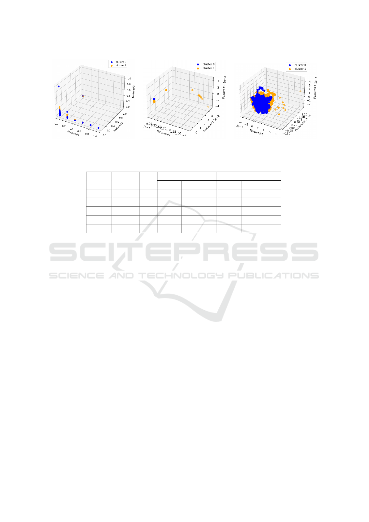
(a) Initial Chunk. (b) Reduced Chunk. (c) Ensemble Chunk.

Figure 1: First Chunk: Comparison of Initial and Transformed Chunks.

Table 3: Clustering Performances of Remaining Chunks.

Chunk TEVR PCs

Initial Ensemble

DB VRC DB VRC

#2 99.8900 100 0.7446 17,361.61 0.5424 24,166.550

#3 99.9998 117 0.4546 1,499.436 0.0851 447,828.401

#4 99.9992 76 0.5948 22,167.308 0.0807 882,006.425

#5 99.9000 100 5.6940 1,110.825 0.6086 14,621.410

#6 99.9100 120 3.256 388.953 0.6528 6,654.930

Next, in Table 4, we also compare the clustering

performances of the reduced and ensemble chunks for

the remaining weeks of data. We notice that the clus-

ter quality has improved signiﬁcantly for the ensem-

ble chunks in most cases, particularly for chunks#3,

#4, and #5. Also, chunk#6 outperforms for VRC

using the ensemble-based dimensionality reduction.

However, ensemble chunk#2 under-performs for both

metrics compared to the reduced chunk#2. The differ-

ences between reduced and ensemble chunks are the

following:

• For chunk#3, #4, and #5, the ensemble-based

chunks outperform with a huge gap in terms of

VRC, whereas, DB outperform with a small gap.

• For chunk#6, only one metric outperforms. VRC

increased with a medium gap for chunk#6 com-

pared to the reduced chunk.

• The ensemble-based dimensionality reduction

under-performs for chunk#2 compared to the re-

duced chunk#2, but with a small and medium gaps

for DB and VRC, respectively.

5.4 Data Labeling

Table 5 presents the number of instances for the two

clusters for the initial and ensemble chunks. As an ex-

ample, regarding chunk#1, out of 9099 instances, we

have 4315 and 4784 instances for clusters 0 and 1, re-

spectively. On the other hand, we have 3733 and 5366

instances for clusters 0 and 1, respectively, for the

ensemble-based initial chunk. Since the ensemble-

based dimensionality reduction approach provided

superior clustering performances for most chunks, we

intend to use its cluster labels as the data labels for all

the chunks.

We also show the mismatch between initial and

ensemble clusters in Table 5. For instance, for chunk

#1, we have 1164 instances from the ensemble chunk

that do not belong to the same cluster as the initial

chunk. We attain the highest mismatch of 1530 in-

stances for chunk #5. For chunk#4, both initial and

ensemble chunks have exact instances for the two

clusters. Moreover, the class distribution is moder-

ately balanced for all the chunks using the ensemble-

based dimensionality reduction method. The highest

imbalance ratio is ≈ 1:3 for chunk #3.

In the future, we will pass only the mismatched

instances of chunk#1 to the human experts to ana-

lyze them and provide us with the ground truth. The

ﬁrst chunk will be used to build the initial classiﬁca-

tion model for service monitoring. Based on an incre-

mental learning approach introduced in (Anowar and

Sadaoui, 2021), we will develop the decision model

gradually using the chunks’ labels.

DeLTA 2022 - 3rd International Conference on Deep Learning Theory and Applications

122

Table 4: Clustering Performances of Reduced and Ensemble Chunks.

Chunk

Reduced Ensemble

DB VRC DB VRC

#2 0.5147 25,727.25 0.5424 24,166.550

#3 0.0906 395,121.06 0.0851 447,828.401

#4 0.0808 881,211.368 0.0807 882,006.425

#5 0.6126 14,294.565 0.6086 14,621.410

#6 0.6420 6,631.924 0.6528 6,654.930

Table 5: Instances in Each Cluster for Each Weekly Chunk.

Chunk

Initial Ensemble

Mismatch

Cluster 0 Cluster 1 Cluster 0 Cluster 1

#1 4315 4784 3733 5366 1164

#2 4144 5936 4310 5770 332

#3 2299 7781 2313 7767 28

#4 4525 5555 4525 5555 0

#5 4791 5289 5556 4524 1530

#6 2702 1832 2306 2228 792

6 CONCLUSIONS AND FUTURE

WORKS

Service monitoring is vital because it allows users

to make proactive decisions when problems arise by

ﬁxing issues and reducing server downtime. The

proposed framework addressed the problems of real-

world data: unlabeled, non-linear and high dimen-

sional time-series data. Nevertheless, service mon-

itoring applications generate time-series data with a

soaring feature space. For this purpose, we devised an

ensemble-based dimensionality reduction approach

based on 1) self-supervised learning to better data

quality, 2) unsupervised dimensionality reduction to

reduce the high data dimensionality, and 3) incremen-

tal dimensionality reduction to improve data labeling.

While implementing this ensemble approach, we

also veriﬁed that a minimal amount of information

was lost throughout the reduction process of the fea-

ture space. We further utilized a time-series data clus-

tering method to assess and compare the quality of

the initial, reduced, and ensemble chunks. The ex-

perimental results showed that higher-quality clusters

(maximum intra-cluster and minimum inter-cluster

distances) had been attained using the ensemble ap-

proach. These high-performing clusters and cluster

labels will be utilized for subsequent decision-making

tasks for the industrial partner.

This current work leads to other research direc-

tions for the same industrial application, as follows:

• Based on the data labels obtained in this study,

we will devise an adaptive ensemble learning ap-

proach to update gradually the service monitoring

classiﬁer with incoming chunks.

• We are also interested in incorporating the

clustering-based outlier detection methods within

the ensemble-based dimensionality reduction ap-

proach to remove outliers from the data.

ACKNOWLEDGEMENTS

We want to express our gratitude to Global AI Ac-

celerator (GAIA) Ericsson, Montreal for collaborat-

ing with us on this research work, the Observability

team for allowing us to access the data, and Fredrik

Hallgren, University College London, UK, for provid-

ing us with the partial implementation of Incremental

KPCA.

REFERENCES

Almotiri, J., Elleithy, K., and Elleithy, A. (2017). Com-

parison of autoencoder and principal component anal-

ysis followed by neural network for e-learning us-

ing handwritten recognition. In 2017 IEEE Long Is-

An Ensemble-based Dimensionality Reduction for Service Monitoring Time-series

123

land Systems, Applications and Technology Confer-

ence (LISAT), pages 1–5. IEEE.

Anowar, F. and Sadaoui, S. (2021). Incremental learn-

ing framework for real-world fraud detection environ-

ment. Computational Intelligence, 37(1):635–656.

Anowar, F., Sadaoui, S., and Dalal, H. (2022). Cluster-

ing quality of a high-dimensional service monitoring

time-series dataset. In 14th International Conference

on Agents and Artiﬁcial Intelligence (ICAART), pages

1–11.

Anowar, F., Sadaoui, S., and Selim, B. (2021). Conceptual

and empirical comparison of dimensionality reduction

algorithms (pca, kpca, lda, mds, svd, lle, isomap, le,

ica, t-sne). Computer Science Review, 40:1–13.

Chin, T.-J. and Suter, D. (2007). Incremental kernel princi-

pal component analysis. IEEE transactions on image

processing, 16(6):1662–1674.

Fan, Z., Wang, J., Xu, B., and Tang, P. (2014). An

efﬁcient kpca algorithm based on feature correla-

tion evaluation. Neural Computing and Applications,

24(7):1795–1806.

Goel, A. and Vishwakarma, V. P. (2016). Gender classiﬁca-

tion using kpca and svm. In 2016 IEEE International

Conference on Recent Trends in Electronics, Informa-

tion & Communication Technology (RTEICT), pages

291–295. IEEE.

Hallgren, F. and Northrop, P. (2018). Incremental ker-

nel pca and the nystrom method. arXiv preprint

arXiv:1802.00043, pages 1–9.

Hawkins, D. M. (2004). The problem of overﬁtting. Jour-

nal of chemical information and computer sciences,

44(1):1–12.

Hoffmann, H. (2007). Kernel pca for novelty detection. Pat-

tern recognition, 40(3):863–874.

Jindal, P. and Kumar, D. (2017). A review on dimension-

ality reduction techniques. International journal of

computer applications, 173(2):42–46.

Joseph, A. A., Tokumoto, T., and Ozawa, S. (2016). Online

feature extraction based on accelerated kernel princi-

pal component analysis for data stream. Evolving Sys-

tems, 7(1):15–27.

Kim, K. I., Franz, M. O., and Scholkopf, B. (2005). Iter-

ative kernel principal component analysis for image

modeling. IEEE transactions on pattern analysis and

machine intelligence, 27(9):1351–1366.

Kumar, A. (2020). Pca explained variance concepts with

python example. https://vitalﬂux.com/pca-explained-

variance-concept-python-example/. Last accessed 12

March 2022.

Lawton, G. (2020). Autoencoders’ example

uses augment data for machine learning.

https://searchenterpriseai.techtarget.com/feature

/Autoencoders-example-uses-augment-data-for-

machine-learning. Last accessed 12 March 2022.

Lim, J., Ross, D. A., Lin, R.-S., and Yang, M.-H. (2004).

Incremental learning for visual tracking. In Advances

in neural information processing systems, pages 793–

800. Citeseer.

Losing, V., Hammer, B., and Wersing, H. (2018). Incre-

mental on-line learning: A review and comparison of

state of the art algorithms. Neurocomputing, Elsevier,

275(1):1261–1274.

Oja, E. (1992). Principal components, minor compo-

nents, and linear neural networks. Neural networks,

5(6):927–935.

Paparrizos, J. and Gravano, L. (2015). k-shape: Efﬁcient

and accurate clustering of time series. In The 2015

ACM SIGMOD International Conference on Manage-

ment of Data, pages 1855–1870.

Pedregosa, F., Varoquaux, G., Gramfort, A., Michel, V.,

Thirion, B., Grisel, O., Blondel, M., Prettenhofer,

P., Weiss, R., Dubourg, V., Vanderplas, J., Passos,

A., Cournapeau, D., Brucher, M., Perrot, M., and

Duchesnay, E. (2011). Scikit-learn: Machine learning

in Python. Journal of Machine Learning Research,

12:2825–2830.

Sanger, T. D. (1989). Optimal unsupervised learning in a

single-layer linear feedforward neural network. Neu-

ral networks, 2(6):459–473.

Spruyt, V. (2014). The curse of dimensionality in classiﬁ-

cation. Computer vision for dummies, 21(3):35–40.

Takeuchi, Y., Ozawa, S., and Abe, S. (2007). An efﬁcient

incremental kernel principal component analysis for

online feature selection. In 2007 International Joint

Conference on Neural Networks, pages 2346–2351.

IEEE.

Tokumoto, T. and Ozawa, S. (2011). A fast incremental ker-

nel principal component analysis for learning stream

of data chunks. In The 2011 International Joint Con-

ference on Neural Networks, pages 2881–2888. IEEE.

Van Der Maaten, L., Postma, E., and Van den Herik, J.

(2009). Dimensionality reduction: A comparative re-

view. J Mach Learn Res, 10(66-71):13.

Verleysen, M. and Franc¸ois, D. (2005). The curse of dimen-

sionality in data mining and time series prediction.

In International work-conference on artiﬁcial neural

networks, pages 758–770. Springer.

Wang, Y., Yao, H., and Zhao, S. (2016). Auto-encoder

based dimensionality reduction. Neurocomputing,

184:232–242.

Zhang, Y. and Li, D. (2013). Cluster analysis by vari-

ance ratio criterion and ﬁreﬂy algorithm. International

Journal of Digital Content Technology and its Appli-

cations, 7(3):689–697.

DeLTA 2022 - 3rd International Conference on Deep Learning Theory and Applications

124