
Comparison of Different Excitation Strategies for Fault Diagnosis of Belt
Drives: Industrial Application Scenarios
Moritz Fehsenfeld
1 a
, Johannes K
¨
uhn
2
, Zygimantas Ziaukas
1 b
and Hans-Georg Jacob
1 c
1
Leibniz University Hannover, Institute of Mechatronic Systems, An der Universit
¨
at 1, Garbsen, Germany
2
Lenze SE, Hameln, Germany
Keywords:
Fault Diagnosis, Machine Learning, Industrial Application, Belt Drives, Mechatronics Systems.
Abstract:
Machine learning (ML) has received a lot of attention in solving fault diagnosis (FD) tasks. As a result, more
and more advanced machine learning algorithms have been developed to increase accuracy. But the system’s
excitation has likewise a high impact on the diagnosis performance and applicability. For this purpose, we
describe different industrial application scenarios and the related set trajectory. They are divided into passive
FD, where normal operation data serves as the input, and active FD, where an optimized excitation is injected.
All scenarios are investigated concerning achievable accuracy and data requirement based on comprehensive
measurements. We demonstrate that in active scenarios a high accuracy of 97.6% combined with a small
number of measurements are obtained by very basic algorithms like a one-nearest neighbor with Euclidean
distance. In passive scenarios, where the FD task is generally harder, the demand for large datasets and more
advanced ML methods increases. In this way, we illustrate how intelligent use of an optimized excitation
strategy leads to feasible, reliable, and accurate fault diagnosis with a broad industrial application spectrum.
1 INTRODUCTION
Fault diagnosis (FD) has seen increasing attention in
the last years. It has the potential to recognize faults
at an early stage and guarantee optimal operation con-
ditions. By this, downtime is decreased, maintenance
costs are reduced and safe operation is ensured. Fol-
lowing this trend, many FD applications of compo-
nents in electromechanical motion systems have been
published in the past. Besides the motor as a major fo-
cus (Kande et al., 2017) other drive elements such as
bearings (AlShorman et al., 2020) and gears (Sharma
and Parey, 2016) are likewise subject to FD.
Belts are a popular drive solution with a wide va-
riety of applications. A proper belt pretension is in-
evitable to operate with high efficiency and low wear.
It is adjusted while commissioning but decreases dur-
ing operation due to changing environments and wear.
For that reason, continuous pretension monitoring en-
sures optimal working conditions. Nevertheless, FD
applications targeting belt drives are rare. (Kang
et al., 2018) predict belt cracks and (Hu et al., 2016)
a
https://orcid.org/0000-0003-2639-7838
b
https://orcid.org/0000-0001-9161-0709
c
https://orcid.org/0000-0001-5605-9704
monitor belt oscillations. The majority of tension
monitoring applications utilize external sensors like
strain gauges (Musselman and Djurdjanovic, 2012;
Bzinkowski et al., 2022) or optical lasers (Khazaee
et al., 2017). These additional sensors are often un-
desired in practice given their extra costs and com-
missioning effort. (Picot et al., 2017) analyze motor
current which does not necessitate extra equipment to
discriminate four tension levels. Consequently, our
proposed FD system to detect a faulty belt tension re-
lies only on standard sensors.
Many contributions in the field of FD focus on the
diagnosis methods. Recently, machine learning (ML)
has attracted great attention. Procedures are catego-
rized into conventional ML and deep learning (DL)
approaches. Conventional ML follows a two-stage
procedure. During feature engineering different sig-
nal processing techniques are applied to facilitate di-
agnosis. These features are handed over to a conven-
tional classification method such as a support vector
machine (Gangsar and Tiwari, 2017) or random for-
est (Toma et al., 2020). Meaningful features are cru-
cial for successful FD, however, require high domain
knowledge. DL approaches omit extensive feature ex-
traction but follow an end-to-end approach where fea-
Fehsenfeld, M., Kühn, J., Ziaukas, Z. and Jacob, H.
Comparison of Different Excitation Strategies for Fault Diagnosis of Belt Drives: Industrial Application Scenarios.
DOI: 10.5220/0011274100003271
In Proceedings of the 19th International Conference on Informatics in Control, Automation and Robotics (ICINCO 2022), pages 177-184
ISBN: 978-989-758-585-2; ISSN: 2184-2809
Copyright
c
2022 by SCITEPRESS – Science and Technology Publications, Lda. All rights reserved
177

tures are learned during training. An outline is pro-
vided by (Thoppil et al., 2021).
Besides the choice of algorithm, the input data
is even more important. A high information content
about the considered task within the data is a basic
prerequisite for successful FD. The selection of ap-
propriate sensors has already been addressed. Mo-
tor current signature analysis (MCSA) and vibrational
analysis are popular among other FD approaches for
electrical drives. An overview of techniques is given
by (Nandi et al., 2005). The restriction to standard
sensor technology does not leave much choice. In
this context, the motor’s motion during diagnosis has
not been considered yet. Generally, passive and ac-
tive FD is distinguished with respect to the set mo-
tion. Passive FD takes normal operation data as input.
The disadvantage is that potential faults can not be
properly diagnosed because the information content is
low. One reason is that high excitations are undesired
during operation. Active FD overcomes this prob-
lem by injecting an additional excitation designed to
maximize diagnosability. It is reported that active FD
yields significantly better performance while it has the
drawback of interfering with the system (Heirung and
Mesbah, 2019). Nevertheless, real-world applications
are rare. Therefore, this work provides an extensive
overview of application scenarios for FD systems.
Our main contributions are: (1) We describe four
typical fault diagnosis scenarios of electromechanical
motion systems without external sensors. (2) We em-
phasize the importance of the set trajectory selection
regarding achievable accuracy and data requirements
for three commonly applied FD algorithms. (3) We
carry out a comprehensive investigation in all scenar-
ios based on measurement data using the example of
belt drives.
The remainder of this work is structured as fol-
lows: Section 2 gives an overview of three common
machine learning algorithms used for fault diagnosis.
Section 3 introduces the belt pretension monitoring
as an example of FD commonly encountered in the
automation industry. Different real-world application
scenarios are described and the testbed used for gath-
ering measurement data is presented. All scenarios
are assessed on extensive datasets in section 4. Con-
clusions and further research directions are given in
section 5.
2 FAULT DIAGNOSIS
ALGORITHMS
ML-based FD is achieved by supervised classifica-
tion of available sensor data x = (x
1
,x
2
,. ..,x
N
) into
healthy and faulty classes y. For this task, a lot of al-
gorithms are proposed in the field of time series clas-
sification (TSC). We select three methods for bench-
marking the classification accuracy in different ap-
plication scenarios. te attempt was made to cover a
broad range of algorithms from basic to advanced.
This section gives insights into all methods.
2.1 One-nearest Neighbor with Distance
Measure
The one-nearest neighbor (1-NN) with a distance
measure is considered a simple baseline approach
which is hard to beat by more advanced methods
(Bagnall et al., 2016). It classifies the data without
transformation. All data are simply stored and a dis-
tance measure assesses the similarity of a new se-
quence to all training samples. The closest sample’s
label is used as prediction following a one-nearest
neighbor approach. Dynamic time warping (DTW)
is an elastic distance measure that accounts for time
shifts and has proven to be suitable for the classifica-
tion of sequential data. Further details can be taken
from (Bagnall et al., 2016). In this work, input data
stems from time and frequency domain. If no data
shift occurs, a simple Euclidean distance (ED) is like-
wise sufficient. A shift can be avoided e.g. in the fre-
quency domain or by restricting the input data. For
the sake of simplicity, we choose 1-NN ED as the
baseline algorithm.
2.2 Statistical Features
Conventional classification algorithms are not suit-
able for raw time series data. Therefore, features are
extracted in the first step. Feature engineering aims to
find features that are as informative as possible with
regard to the target variable. This step is crucial for
high accuracy. Statistical features that summarize cer-
tain characteristics of the underlying time series are
a frequently chosen possibility (Fulcher and Jones,
2014). A collection of common statistical features ap-
plied in this work is given in Table 1. The advantage
of simple feature functions such as mean F
1
, maxi-
mum F
5
minimum F
6
, or energy F
13
is a decent level
of interpretability. The classifier’s decision is thereby
comprehensible promoting the general acceptance of
machine learning in the industry.
A random forest classifier has proven to be effec-
tive in combination with statistical features (Fehsen-
feld et al., 2020). It consists of multiple Classification
and Regression Trees (CART) described by (Breiman,
2001). Decision trees are trained from the root to mul-
tiple leaves connected by nodes. At each node, the
ICINCO 2022 - 19th International Conference on Informatics in Control, Automation and Robotics
178
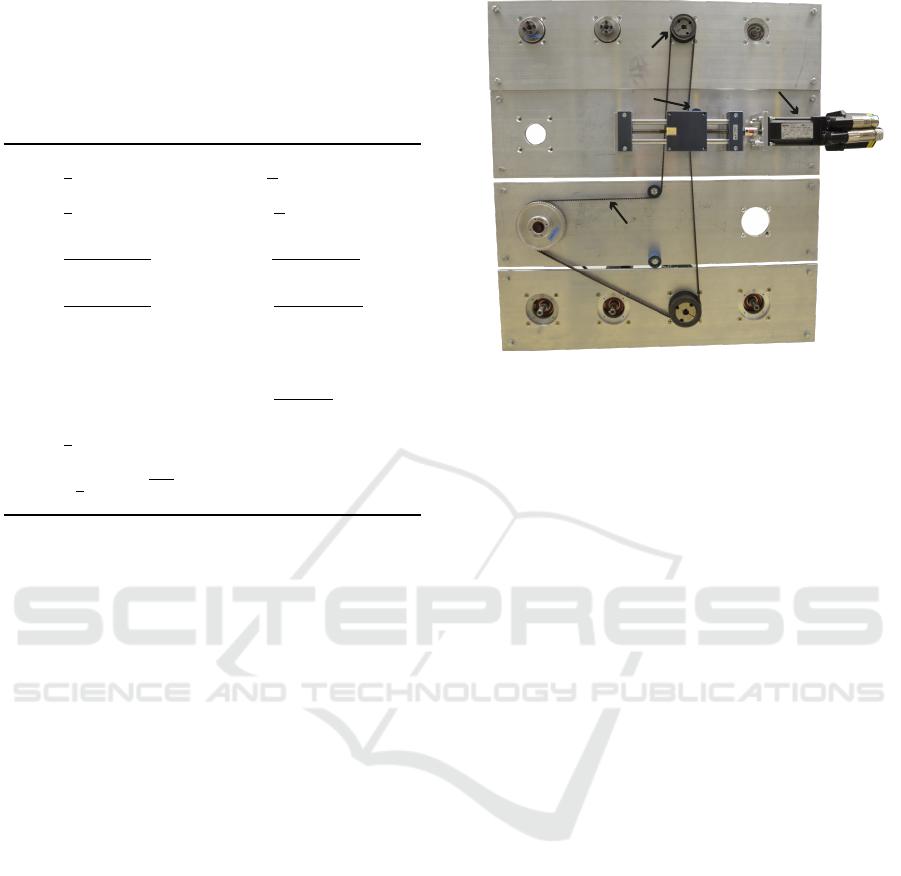
Table 1: Overview of feature functions F
i
. In the time do-
main the sequence consist of a value x
i
and a related time t
i
at each step ∀i ∈ {1, ..., L}. Transformed by FFT into fre-
quency domain the sequence comprises of an amplitude a
i
and a related frequency f
i
for ∀i ∈ {1,. .., K}.
Time domain Frequency domain
F
1
=
1
L
∑
L
i=1
x
i
F
9
=
1
K
∑
K
i=1
a
i
F
2
=
1
L
∑
L
i=1
(x
i
− F
1
)
2
F
10
=
1
K
∑
K
i=1
(a
i
− F
9
)
2
F
3
=
∑
L
i=1
(x
i
−F
1
)
3
L·F
3
2
F
11
=
∑
K
i=1
(a
i
−F
9
)
3
k·F
3
10
F
4
=
∑
L
i=1
(x
i
−F
1
)
4
L·F
4
2
F
12
=
∑
K
i=1
(a
i
−F
9
)
4
K·F
4
10
F
5
= min(x) F
13
=
∑
K
i=1
a
2
i
F
6
= max(x) F
14
=
∑
K
i=1
a
i
· f
i
∑
K
i=1
a
i
F
7
=
1
L
∑
L
i=1
|x
i
|
F
8
=
1
L
∑
L
i=1
p
|x
i
|
2
feature space is further split until regions exist where
classification can be done. (Breiman, 2001) gives de-
tailed information about the method. This approach is
further referred to as SF+RF.
2.3 Minirocket
Minirocket (MINImally RandOm Convolutional
KErnel Transform) proposed by (Dempster et al.,
2021) is a fast classification algorithm which achieves
state-of-the-art performance on a wide variety of TSC
problems in the UCR time series classification archive
(Dau et al., 2018). The time series is transformed by a
large (by default n
f
= 10000) number of random con-
volutional kernels. The feature space K = (k
1
,. ..k
n
f
)
is obtained by calculating the proportion of positive
values for each kernel transformation. Details on the
kernels are reported in (Dempster et al., 2021). A lin-
ear ridge regression classifier is used as recommended
by the authors. For this purpose, the linear regression
ˆy = β
0
+ β
1
k
1
+ ... + β
n
f
k
n
f
(1)
is utilized, where ˆy is the predicted target variable.
The coefficients β
i
are estimated based on available
target variables y
i
by
ˆ
β = min
β
n
obs
∑
i=1
y
i
− β
0
−
n
f
∑
j=1
β
j
k
i, j
2
+ λ
n
f
∑
j=1
β
2
j
, (2)
where the first term is the residual sum of squares and
the second term is a shrinkage penalty forcing β
j
to
be close to zero. λ is the tuning parameter trading off
the two terms. (James et al., 2014)
belt
roller
powered pulley
servo motor
(belt tension)
Figure 1: Belt drive used for evaluation of different appli-
cation scenarios of belt pretension fault diagnosis.
3 FAULT DIAGNOSIS OF BELT
DRIVES
Electromechanical motion systems are applied in
many industrial fields. High reliability and efficiency
of all components involved are vital for safe and ef-
ficient operation. Toothed belts are popular drive el-
ements because they combine the capability of high
acceleration, smooth running characteristics, and high
precision for point-to-point motions (Perneder and
Osborne, 2012). Diagnosing a belt drive’s pretension
serves as an FD example to introduce real-world ap-
plication scenarios. At this point, it is highlighted that
the selection of input data is not restricted to this case
but should be considered for every FD system.
The validation of all scenarios is based on mea-
surement data. Therefore, the experimental setup is
introduced first. After that, we demonstrate how to
realize active and passive FD in this example.
3.1 Experimental Setup
A belt drive with adjustable pretension is used to
gather measurement data. It is depicted in Figure
1. There are four pulleys connected by a toothed
belt with AT-5 profile and a total length of l = 2 m.
The upper pulley is powered by a servomotor with
a rated torque of M
0
= 1.2 Nm and a rated power of
P
0
= 1.2kW. The servomotor is equipped with stan-
dard sensors that are available in real-world applica-
tions:
• position ϕ
act
(and derivatives
˙
ϕ
act
,
¨
ϕ
act
),
• torque M
act
,
• temperature ϑ.
Comparison of Different Excitation Strategies for Fault Diagnosis of Belt Drives: Industrial Application Scenarios
179

Consequently, broad applicability is ensured by in-
volving only standard sensors.
Another servo motor adjusts the belt tension that
moves a roller attached to a linear axis. The servo-
motor’s position correlates with the belt pretension.
A characteristic curve between the servomotor’s po-
sition and the belt tension force F
belt
is created which
is only used to label the measurement data and not
for prediction. The pretension force ranges from
F
belt,min
= 40 N to F
belt,max
= 200 N. Afterwards, it
is discretized into n
c
= 5 equally-spaced classes.
3.2 Application Scenarios
The diagnosis solely relies on the input data gathered
from the machine regardless of the downstream algo-
rithm. Obviously, the input data has a high impact on
the diagnosis performance. In many real-world appli-
cations, there is a certain amount of freedom in de-
signing the FD system which will be carved out in the
section below. Set trajectories for passive and active
scenarios are defined and measurements are gathered.
Random samples of each class are shown in Figure 2
and discussed below.
3.2.1 Passive Fault Diagnosis
Passive FD takes only normal operation data as in-
put to the algorithm. During normal operation, the
servo motor fulfills specific tasks by following point-
to-point motions. Jerk-limited trajectories (JLT) are
the industrial standard for this purpose. The trajec-
tory between the start ϕ
start
and end position ϕ
end
is
designed in advance during path planning. Matching
set position ϕ
set
(t) and set velocity
˙
ϕ
set
(t) are calcu-
lated. A rectangular-shaped and thereby limited set
jerk
...
ϕ
set
(t) and the associated trapezoidal set acceler-
ation is characteristic for JLT. The shape is defined by
the maximum values of jerk
...
ϕ
max
, acceleration
¨
ϕ
max
,
velocity
˙
ϕ
max
and the distance d = ϕ
end
− ϕ
start
. The
outcome is a smooth trajectory between ϕ
start
and x
end
hereby limiting the excitation of oscillations initiated
by the set trajectory.
In the case of passive FD, it is inevitable to analyze
JLT whether a fault has occurred. Two scenarios have
been chosen which are feasible in practice.
Random Test Trajectory. During operation a large
variety of JLT can be the result to fulfill the designated
tasks. Therefore, all kind of JLT must be analyzed
to be capable of fault diagnosis at any time. In this
scenario, a dataset is created where all characteristic
JLT parameters are chosen randomly and uniformly
distributed as follows:
d ∼ U(100 deg,2000 deg),
˙
ϕ
max
∼ U(1000deg /s,7000 deg/s),
¨
ϕ
max
∼ U(1000deg /s
2
,6000 deg/s
2
),
...
ϕ
max
∼ U(6000deg /s
3
,60 000 deg/s
3
). (3)
Consequently, the input data of the FD algorithm has
a high variety. Random sections of the trajectories
are selected to cut all samples to equal length. In this
manner, a sliding window with fixed size of t
win
= 1s
is imitated. Examples are shown in Figure 2a. All set
trajectories differ making it hard to recognize patterns
between the classes with the naked eye.
Fixed Test Trajectory. During operation, a motion
can occur regularly when accomplishing a repeating
task e.g. moving a lifting station from the ground to
the first level. By choosing a certain JLT the vari-
ety of the input data is eliminated. The characteris-
tic pattern of the FD target is now potentially better
visible because the input variety significantly drops.
The drawback is that potential faults can only be de-
tected during this typical motion. In the case of faulty
belt tension, this drawback seems acceptable since the
pretension reduces gradually due to wear. But a sud-
den loss remains possibly undetected.
There are many potential trajectories for this sce-
nario. Two JLT are compared to evaluate the impor-
tance of trajectory selection. Trajectory T
1
is chosen
to be comparatively fast, while trajectory T
2
has re-
duced velocity. The parameters are chosen as follows:
d
1
= 700deg,
˙
ϕ
max,1
= 7000deg /s,
¨
ϕ
max,1
= 50000 deg/s,
...
ϕ
max,1
= 200000 deg/s
3
.
d
2
= 2500deg,
˙
ϕ
max,2
= 1000deg /s,
¨
ϕ
max,2
= 50000 deg/s,
...
ϕ
max,2
= 200000 deg/s
3
.
Trajectory T
2
is visualized in Figure 2b. The set tra-
jectory is the same for all runs which can be seen in
the rotational speed signal. No big differences are vis-
ible between the classes indicating that the controller
is able to follow the set value. The torque acts as the
control variable. Slight deviations between the classes
can be detected. All findings apply for trajectory T
1
as well.
3.2.2 Active Fault Diagnosis
In an active FD scenario, input data is not restricted to
JLT but every motion is possible. Therefore, the first
task is designing an optimal input sequence leading
to an easy diagnosis of the considered faults. In the
ICINCO 2022 - 19th International Conference on Informatics in Control, Automation and Robotics
180
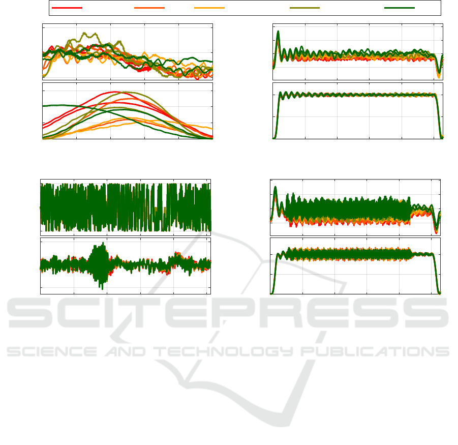
very loose loose slightly loose slightly tight tight
0
0.2
0.4
M
act
in Nm
0 0.2 0.4 0.6 0.8
time in s
0
1000
2000
3000
_'
act
in deg/s
(a) Random test trajectory.
0
0.2
0.4
0.6
M
act
in Nm
0 0.5 1 1.5 2 2.5
time in s
0
500
1000
_'
act
in deg/s
(b) Fixed test trajectory (T
2
).
-0.2
0
0.2
M
act
in Nm
0 0.1 0.2 0.3 0.4 0.5
time in s
-1
0
1
_'
act
in deg/s
(c) Optimized excitation at standstill.
0
0.2
0.4
0.6
M
act
in Nm
0 0.5 1 1.5 2 2.5
time in s
0
500
1000
_'
act
in deg/s
(d) Superposition during operation.
Figure 2: The actual torque M
act
and the actual rotational speed
˙
ϕ
act
are shown for all scenarios in the time domain. Random
observations for each class (n
c
= 5) are drawn.
case of belt drives, multi-frequency excitations (MFE)
have proven successful (Fehsenfeld et al., 2020). It is
a superposition of n
freq
sine signals
M
add
(t) = A ·
n
freq
∑
i=0
sin(2π f
i
t + φ
i
), (4)
having different frequencies f
i
and phases φ
i
. All
sine signals are phase-shifted to avoid extreme values
making the signal as compact as possible. The each
phase φ
i
is chosen according to (Schroeder, 1970).
The MFE can further be optimized by adjusting the
amplitude A and the frequency content f
i
.
Two different application scenarios are considered
for active FD using an MFE as an auxiliary signal by
adding it as torque offset M
add
. First, the MFE is in-
jected at standstill. In the other scenario, it is applied
during operation.
Optimized MFE at Standstill. In practice, there
might be natural stops of production overnight or dur-
ing waiting periods until the next motion is triggered.
In these situations, the test excitation can easily be
applied. Since the normal operation is not affected,
constraints regarding the auxiliary signal are small.
As long as the servo drive and the mechanics are not
damaged, the impact is irrelevant.
A heuristic tuning of all MFE parameters is car-
ried out in the design stage. The frequency content
is observed to be optimal with n
freq
= 256 frequen-
cies ranging from f
min
= 1.9531 Hz to f
max
= 500 Hz.
The length of the MFE is set to t
max
= 0.512 s ensur-
ing an integral multiple of the period duration of each
frequency to avoid spectral leakage when transform-
ing to frequency domain. The amplitude of all sines
is set to A = 0.015Nm. The optimized MFE is shown
in Figure 2c as torque signal M
act
. There are no dif-
ferences between the belt classes since it is a set sig-
nal. The rotational speed
˙
ϕ
act
includes the system’s
response. In the time domain, only slight deviations
are visible. A fast Fourier transform (FFT) is applied
to obtain the frequency domain. A small but highly
reproducible shift of characteristic frequencies across
the classes can be observed in Figure 3.
While the possibilities to design an appropriate
auxiliary signal are many, the biggest drawback is
Comparison of Different Excitation Strategies for Fault Diagnosis of Belt Drives: Industrial Application Scenarios
181

very lo os e loose slightly loose
slightly tight tight
0 100 200 300 400
frequency in Hz
-80
-60
-40
-20
amplitude in dB
Figure 3: Frequency domain of rotational speed
˙
ϕ
act
when
excited by optimized MFE at standstill.
the fact that the operation must be interrupted. If
no pauses in the process are possible or desired, the
auxiliary signal must be injected during operation to
make active FD viable in this case.
Optimized MFE during Operation. If the auxil-
iary signal is injected into a motion it is desirable to
keep its impact at a minimum. Especially the ampli-
tude A has a high effect and must be chosen as small
as possible. This leads to a trade-off between perfor-
mance and disturbance since a higher amplitude nor-
mally leads to better diagnosability. A heuristic tun-
ing is done to balance this trade-off. The frequency
content is found to be optimal with n
freq
= 4 from
f
min
= 100 Hz to f
max
= 300 Hz. The amplitude is
set to A = 0.02Nm and the total excitation length is
t
max
= 1.921 s. This MFE superposes the normal op-
eration in the phase of constant velocity. The fixed
trajectory T
2
is chosen for direct comparison to a pas-
sive scenario. The superposition is visible in both
torque and rotational speed signals in Figure 2d start-
ing at t ≈ 0.2 s. The maximum speed error
˙
ϕ
set
−
˙
ϕ
act
is increased by approximately 9 % due to superposi-
tion compared to the original motion. If no task is
performed that requires high path accuracy this seems
acceptable in many real-world applications.
4 EXPERIMENTAL RESULTS
For all scenarios training and test datasets are created.
Both datasets are independently recorded. The train-
ing and test dataset size for the random trajectory sce-
nario is n
obs,1
= 10000, for all other scenarios it is
n
obs,2
= 1000.
All datasets are used to evaluate two different as-
pects of FD. The ability to reliably recognize faults
is the key factor for successful FD. The classifica-
tion accuracy is hence assessed in the first step. Fur-
thermore, a big problem in real-world applications is
that datasets are usually scarce because data gathering
and labeling are associated with large human effort.
The number of required measurements is desirably as
small as possible and therefore additionally investi-
gated. An overview of all results on the test dataset is
given in Table 2 and will be further discussed subse-
quently.
4.1 Achievable Accuracy
The classification results of all algorithms introduced
in section 2 can be seen in Table 2. As expected, the
accuracy in active FD scenarios is higher compared
to passive FD scenarios. In both active scenarios, the
accuracy is notably above 90% accomplishing a near-
perfect outcome. In a passive scenario, the accuracy
drops significantly. When considering a fixed test tra-
jectory the achievable performance depends on its se-
lection. Trajectory 2 is more suitable for FD than tra-
jectory 1 regardless of the algorithm. In the case of
random trajectories by definition no selection is nec-
essary. All kinds of trajectories are present whereby
some are better suitable than others. The result is a
maximum accuracy of approximately 90% requiring
a massive amount of measurements.
The comparison of selected FD algorithms yields
expectable results. The state-of-the-art classifier
minirocket outperforms 1-NN ED and SF+RF in all
scenarios. It can be concluded that the findings in
both active scenarios do not differ much and basic
algorithms perform equally well. In the passive sce-
narios where classification is more difficult minirocket
shows its capabilities.
4.2 Data Requirements
The required amount of data is determined by grad-
ually reducing the training dataset size. The results
Table 2: Maximum achievable test accuracy Acc
max
(top)
and minimum dataset size n
min
(below). The belt tension is
discretized into n
c
= 5 classes.
Scenario 1-NN ED SF + RF Minirocket
MFE
97.6 %
143
98 %
143
99.7%
484
Superposed
traj.
89.8 %
725
95.6 %
310
99.2%
502
Fixed test
traj. 1
74.7 %
660
87.8 %
690
97.4%
930
Fixed test
traj. 2
80.5 %
660
93.8 %
725
99.1%
930
Random
traj.
50.1 %
8860
81.5 %
7860
89.7%
7970
ICINCO 2022 - 19th International Conference on Informatics in Control, Automation and Robotics
182
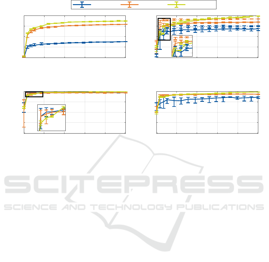
1-NN ED SF + RF minirocket
2000 4000 6000 8000 10000
number of ob servations
20
40
60
80
100
accuracy in %
(a) Random test trajectory.
200 400 600 800
number of ob servations
20
40
60
80
100
accuracy in %
(b) Fixed test trajectory. The solid line is trajectory 1
and dashed line is trajectory 2.
200 400 600 800
number of ob servations
20
40
60
80
100
accuracy in %
(c) Optimized excitation at standstill.
200 400 600 800
number of ob servations
20
40
60
80
100
accuracy in %
(d) Superposition during operation.
Figure 4: Test accuracy over number of training observations in all scenarios and FD algorithms. The training dataset is drawn
five times independently from all training samples while test dataset is kept constant. Errorbars show the scattering.
for data requirements are depicted in Figure 4. In all
cases, a convergence behavior towards the maximum
achievable test accuracy is observed. It can be con-
cluded that enough data was gathered. The required
dataset size n
min
is calculated as the smallest number
of observations needed to achieve 99 % of maximum
test accuracy in each scenario. The results are added
to Table 2.
Again, active FD scenarios show advantageous
properties. Small datasets are sufficient to reach
a high accuracy regardless of the algorithm. Ba-
sic methods generally require fewer data while
minirocket tends to require more data. It can be no-
ticed in Figure 4c and Figure 4b that SF+RF even out-
performs minirocket on small dataset sizes n
obs
< 200.
The superposition of a JLT has a positive effect com-
pared to the original motion. The data requirement
notably decreases and the accuracy improves in par-
ticular for 1-NN ED, while for SF+RF and minirocket
it is already on a high level.
In passive FD scenarios, the selection of the al-
gorithm is of greater importance as large differences
are observed. 1-NN ED shows worst results followed
by SF+RF, whereas minirocket yields a high accu-
racy for both fixed trajectories. A random trajectory
scenario seems infeasible in practical applications be-
cause of the massive amount of data (n
obs
> 7500)
needed.
5 CONCLUSIONS AND FUTURE
WORK
In this work, different FD application scenarios of
electromechanical drive systems are described and
examined. They are divided into passive scenarios
which rely on jerk-limited trajectories and active sce-
narios where an MFE is injected. We demonstrate
how an additional excitation leads to several advan-
tages: By using an optimized MFE at standstill, even
a very basic algorithm like 1-NN ED achieves a high
accuracy of 97.6% while only n
obs
≈ 143 number
of training samples are required. Furthermore, the
applicability of basic methods promotes secondary
objectives like interpretability. In passive scenarios
classification becomes more difficult. The accuracy
drops below 90% in many cases. In this case, the
state-of-the-art classifier minirocket stands out with
high accuracy, but requiring a significantly increased
amount of data (n
obs
> 800). A random trajectory
scenario seems practically infeasible due to low ac-
curacy (Acc < 90 %) and massive data requirement
(n
obs
> 7500). As a result, active FD is preferred over
passive FD. The intelligent use of optimized excita-
tions leads to feasible, reliable, and accurate fault di-
agnosis in a broad application spectrum.
Comparison of Different Excitation Strategies for Fault Diagnosis of Belt Drives: Industrial Application Scenarios
183

Active fault diagnosis is lacking practical exam-
ples. The design of appropriate auxiliary signals for a
broad range of FD applications is still open. Further
research in this direction has the potential to enable
safe and economical FD in real-world applications.
ACKNOWLEDGEMENTS
The authors of the Institute of Mechatronic Systems
would like to thank Lenze SE for enabling the coop-
erative project.
REFERENCES
AlShorman, O., Irfan, M., Saad, N., Zhen, D., Haider, N.,
Glowacz, A., and AlShorman, A. (2020). A Review
of Artificial Intelligence Methods for Condition Mon-
itoring and Fault Diagnosis of Rolling Element Bear-
ings for Induction Motor.
Bagnall, A., Lines, J., Bostrom, A., Large, J., and Keogh,
E. (2016). The great time series classification bake
off: a review and experimental evaluation of recent
algorithmic advances. Data Mining and Knowledge
Discovery.
Breiman, L. (2001). Random forests. Machine Learning,
45(1):5–32.
Bzinkowski, D., Ryba, T., Siemiatkowski, Z., and Rucki,
M. (2022). Real-time monitoring of the rubber belt
tension in an industrial conveyor. Reports in Mechan-
ical Engineering, 3(1):1–10.
Dau, H. A., Keogh, E., Kamgar, K., Yeh, C.-C. M., Zhu,
Y., Gharghabi, S., Ratanamahatana, C. A., Yanping,
Hu, B., Begum, N., Bagnall, A., Mueen, A., Batista,
G., and Hexagon-ML (2018). The ucr time series
classification archive. URL:https://www.cs.ucr.edu/
∼
eamonn/time series data 2018/.
Dempster, A., Schmidt, D. F., and Webb, G. I. (2021).
MINIROCKET: A Very Fast (Almost) Determinis-
tic Transform for Time Series Classification. Pro-
ceedings of the 27th ACM SIGKDD Conference on
Knowledge Discovery & Data Mining, pages 248–
257. arXiv: 2012.08791.
Fehsenfeld, M., K
¨
uhn, J., Wielitzka, M., and Ortmaier,
T. (2020). Tension Monitoring of Toothed Belt
Drives Using Interval-Based Spectral Features. IFAC-
PapersOnLine, 53(2):738–743.
Fulcher, B. D. and Jones, N. S. (2014). Highly comparative
feature-based time-series classification. IEEE Trans-
actions in Knowledge and Data Engineering, pages
3026–3037.
Gangsar, P. and Tiwari, R. (2017). Comparative investiga-
tion of vibration and current monitoring for prediction
of mechanical and electrical faults in induction mo-
tor based on multiclass-support vector machine algo-
rithms. Mechanical Systems and Signal Processing,
94:464–481.
Heirung, T. A. N. and Mesbah, A. (2019). Input design
for active fault diagnosis. Annual Reviews in Control,
47:35–50.
Hu, Y., Yan, Y., Wang, L., and Qian, X. (2016). Non-
contact vibration monitoring of power transmission
belts through electrostatic sensing. IEEE Sensors
Journal, 16(10):3541–3550.
James, G., Witten, D., Hastie, T., and Tibshirani, R. (2014).
An Introduction to Statistical Learning: With Applica-
tions in R. Springer, New York, NY, 1 edition.
Kande, M., Isaksson, A., Thottappillil, R., and Taylor, N.
(2017). Rotating electrical machine condition moni-
toring automation—a review. Machines, 5(4):24.
Kang, T., Yang, C., Park, Y., Hyun, D., Lee, S. B., and
Teska, M. (2018). Electrical monitoring of mechanical
defects in induction motor-driven v-belt–pulley speed
reduction couplings. IEEE Transactions on Industry
Applications, 54(3):2255–2264.
Khazaee, M., Banakar, A., Ghobadian, B., Mirsalim, M. A.,
Minaei, S., and Jafari, S. M. (2017). Detection of
inappropriate working conditions for the timing belt
in internal-combustion engines using vibration signals
and data mining. Proceedings of the Institution of Me-
chanical Engineers, Part D: Journal of Automobile
Engineering, 231(3):418–432.
Musselman, M. and Djurdjanovic, D. (2012). Tension mon-
itoring in a belt-driven automated material handling
system. CIRP Journal of Manufacturing Science and
Technology, 5(1):67 – 76.
Nandi, S., Toliyat, H. A., and Li, X. (2005). Condition
monitoring and fault diagnosis of electrical motors—a
review. IEEE Transactions on Energy Conversion,
20(4):719–729.
Perneder, R. and Osborne, I. (2012). Handbook Timing
Belts. Springer Berlin Heidelberg.
Picot, A., Fournier, E., R
´
egnier, J., TientcheuYamdeu, M.,
Andr
´
ejak, J., and Maussion, P. (2017). Statistic-
based method to monitor belt transmission looseness
through motor phase currents. IEEE Transactions on
Industrial Informatics, 13(3):1332–1340.
Schroeder, M. (1970). Synthesis of low-peak-factor sig-
nals and binary sequences with low autocorrelation
(corresp.). IEEE Transactions on Information Theory,
16(1):85–89.
Sharma, V. and Parey, A. (2016). A Review of Gear Fault
Diagnosis Using Various Condition Indicators. Pro-
cedia Engineering, 144:253–263.
Thoppil, N. M., Vasu, V., and Rao, C. S. P. (2021). Deep
Learning Algorithms for Machinery Health Prognos-
tics Using Time-Series Data: A Review. Journal of
Vibration Engineering & Technologies.
Toma, R. N., Prosvirin, A. E., and Kim, J.-M. (2020).
Bearing Fault Diagnosis of Induction Motors Using a
Genetic Algorithm and Machine Learning Classifiers.
Sensors, 20(7):1884.
ICINCO 2022 - 19th International Conference on Informatics in Control, Automation and Robotics
184
