
Estimating the Optimal Number of Clusters from Subsets of Ensembles
Afees Adegoke Odebode, Allan Tucker, Mahir Arzoky and Stephen Swift
Brunel University, London, U.K.
Keywords:
Ensemble Clustering, Subset Selection, Cluster Analysis, Number of Clusters.
Abstract:
This research estimates the optimal number of clusters in a dataset using a novel ensemble technique - a
preferred alternative to relying on the output of a single clustering. Combining clusterings from different
algorithms can lead to a more stable and robust solution, often unattainable by any single clustering solution.
Technically, we created subsets of ensembles as possible estimates; and evaluated them using a quality metric
to obtain the best subset. We tested our method on publicly available datasets of varying types, sources and
clustering difficulty to establish the accuracy and performance of our approach against eight standard methods.
Our method outperforms all the techniques in the number of clusters estimated correctly. Due to the exhaustive
nature of the initial algorithm, it is slow as the number of ensembles or the solution space increases; hence, we
have provided an updated version based on the single-digit difference of Gray code that runs in linear time in
terms of the subset size.
1 INTRODUCTION
Finding the number of clusters in a dataset remains
a largely unsolved problem in cluster analysis since
there is often no clear definition of what constitutes a
“cluster”. Clustering is assigning similar data points
to the same cluster and dissimilar points to different
clusters without any prior knowledge of the members’
labels (Jain et al., 1999). It can also be described
as an application that determines partitions based on
distance and correlation metrics (Swift et al., 2007).
The clustering process often involves determining the
number of clusters by learning from similarity or dis-
similarity between objects or points in the dataset.
Learning or estimating clusters in datasets is a sub-
tle way of unravelling the pattern or the underlying
structure in the dataset from where other analyses can
commence.
This paper employed a novel ensemble method to
estimate the number of clusters in datasets. Ensem-
ble clustering, first introduced by (Strehl and Ghosh,
2002), is a technique that improves clustering perfor-
mance by generating multiple partitions of a dataset
and combining them to create a summary clustering
solution. Ensemble methods have various applica-
tions in classification techniques (Giacinto and Roli,
2001), (West et al., 2005), and due to its success-
ful application, attempts have been made to apply
the same model in unsupervised learning. Two main
questions that often arise in a clustering ensemble are:
(i) What is the best way of generating the cluster-
ings and combining them into representative so-
lutions while maintaining diversity and promot-
ing accuracy?
(ii) What is the optimal way of identifying the best
solution from the pool of representative solu-
tions(subsets)?
We attempt to answer both questions by creating
all possible subsets of ensembles and generating an
agreement matrix between outputs from the differ-
ent clustering algorithms. The agreement matrix con-
tains cluster similarity from the clusterings for each
value of the number of clusters (k). The subset with
the maximum agreement as determined by our quality
function is the best subset, and the best subset’s index
is the number of clusters in the dataset. An exhaus-
tive search for the best subset can be computationally
intensive as the clusterings increase. Therefore, we
used a technique that maps outputs from the agree-
ment matrix to Gray codes
1
successive members to
create subsets. We provided a run-time of both im-
plementations (quality and update quality). The re-
sults show that our approach is accurate for different
datasets, distributions, and datasets with outliers com-
pared with similar methods. Some methods described
1
Gray code is the weighted code where only one-bit
changes for every two consecutive members.
Odebode, A., Tucker, A., Arzoky, M. and Swift, S.
Estimating the Optimal Number of Clusters from Subsets of Ensembles.
DOI: 10.5220/0011275000003269
In Proceedings of the 11th International Conference on Data Science, Technology and Applications (DATA 2022), pages 383-391
ISBN: 978-989-758-583-8; ISSN: 2184-285X
Copyright
c
2022 by SCITEPRESS – Science and Technology Publications, Lda. All rights reserved
383

below depend on specific data distribution, for exam-
ple, Gaussian distribution and may suffer from over-
fitting. Our approach does not because the estimated
clusters rely on the agreement matrix generated from
multiple clusterings.
Cluster analysis is essential in exploratory data
analysis and data cleaning with many practical ap-
plications, which includes: character recognition (Ar-
ica and Yarman-Vural, 2001), tissue segmentation and
tumour identification (Vishnuvarthanan et al., 2016),
also in applications involving astronomical data clas-
sification (Zhang and Zhao, 2004), and more recently
in bioinformatics and related applications (Higham
et al., 2007). Our primary motivation for this work
is two-fold: accuracy and effort. Accuracy is mea-
sured as the correctly estimated number of clusters
compared with similar metrics, and effort is how fast
the prediction takes or the runtime. It has been shown
(Ayed et al., 2018) that the average Weighted Kappa
(W
k
)
2
between pair of inputs highly correlates to the
average Weighted Kappa (W
k
) of each input compared
to the expected number of clusters (gold standard).
We can thus infer that selecting the best subset (sub-
set with the highest average Weighted Kappa) should
strongly correlate to the gold standard without know-
ing it beforehand. Therefore, it can be used as a proxy
for the gold standard. The following are some of our
contributions:
• We design a selection scheme that searches for the
subset/solution from the ensemble of input clus-
tering techniques.
• We formulate an objective function that deter-
mines the quality of a subset and finds the subset
that optimises the objective function(quality).
• We establish a mathematical framework for the
quality metrics. The metrics allow larger subsets
to be scored in parity with smaller subsets using
the threshold.
The rest of this paper is organised as follows: Sec-
tion 2 contains a review of the literature and an intro-
duction to some standard methods used in estimating
the number of clusters in datasets. Section 3 lays out
the framework of our ensemble technique, whilst Sec-
tion 4 describes the datasets used for the experiments.
The experimental detail is in section 5 and the results
of the experiments and their comparison with exist-
ing methods are in Section 6. The conclusions and
recommendations are in section 7.
2
Weighted Kappa is a metric that compares expected
accuracy with observed accuracy based on the agreement
between the two, and it is equivalent to the Adjusted Rand.
2 ESTIMATING THE NUMBER
OF CLUSTERS
There are several methods for determining the num-
ber of clusters in datasets; most are dated. We selected
a range of standard methods and indices to compare
with our method. The first category of methods we
used are those that cluster datasets and then report the
number of clusters; essentially, they are clustering al-
gorithms. We consider three methods in this category.
First, X-means (Pelleg et al., 2000) for example, pro-
vides a framework for estimating the number of clus-
ters in datasets using k with the best Bayesian Infor-
mation Criterion (Kass and Wasserman, 1995) score.
However, X-means assumes that the width of the co-
variances is identical and spherical, thus limiting the
method to specific data distribution. X-means is one
of the methods we used in generating the initial clus-
terings. (Hamerly and Elkan, 2003) proposed the G-
means algorithm. The algorithm grows the value of
k starting with a small number of centres and tests if
the data is from a Gaussian distribution using a statis-
tical test. Those not from Gaussian distribution are
split into two repeatedly until all assume Gaussian
distribution. Although G-means works well, if the
data is well separated, it can encounter difficulty with
overlapping data. In this category, we also consid-
ered the Expectation-Maximisation (EM) algorithm.
Unlike distance-based and hard clustering algorithms
such as k-means, EM constructs statistical models of
the data and accommodates categorical and continu-
ous data fields with varying degrees of data member-
ship in multiple clusters.
The second category of methods we reviewed
against our ensemble techniques are the nineteen clas-
sical methods from the R’s nbclust
3
package (Char-
rad et al., 2014); we will explain a few of the meth-
ods here and report on the top five based on the
outputs. One of the methods is Gap statistics. It
compares the total intra-cluster variation for differ-
ent values of clusters with their expected values un-
der specific distribution, for example, the null ref-
erence distribution. Although it is good at identify-
ing well-separated clusters, it can sometimes overes-
timate the number of clusters for exponential distri-
butions (Sugar and James, 2003). We also compared
our method with the Silhouettes (Rousseeuw, 1987)
technique. The Silhouettes technique depends on par-
titions from the clustering and the collection of prox-
3
nbclust provides 30 indices for determining the num-
ber of clusters and proposes to the user the best clustering
scheme from the different results obtained by varying all
combinations of number of clusters, distance measures, and
clustering methods.
DATA 2022 - 11th International Conference on Data Science, Technology and Applications
384

imities between the objects to construct the Silhou-
ette plot. Lastly, we included the Calinski Harabasz
(Calinski and Harabasz, 1974) (CH) index, Ball (Ball
and Hall, 1965), Ratkwosky (Ratkowsky and Lance,
1978), Krzanowski Lai (Krzanowski and Lai, 1988),
and Milligan (Milligan, 1981) as implemented in R’s
nbclust package (Charrad et al., 2014) . The Calinski
index, like all the other indices, maximises the CH in-
dex and is computed as shown in equation 1. Where
k is the number of clusters, n is the number of data
points, B
k
is the between clusters sum of squares, and
C
k
is the within-cluster sum of squares. The rest of
the methods in this category seek to maximise a value
or an index. We selected the best five of the methods,
and the results are as presented in section 7.
CH(k) =
B
k
/(k −1)
C
k
/(n −k)
(1)
In summary, the common theme of the above
methods is that they are all based on a single input
method, such as k-means or hierarchical clustering,
for generating the clusterings. The current method ex-
plores multiple clusterings to increase diversity, thus
encouraging inputs from both strong and weak clus-
terings for the optimal estimate. However, both ap-
proaches seek to maximise a metric defined as a func-
tion of the number of clusters. The index that corre-
sponds to the maximum value of the metric as shown
in Figure 1 is the estimated number of clusters in the
dataset. None of the approaches are guaranteed to
perform well in all situations; they tend to over-fit,
under-fit, or are too computationally costly, but we
are optimistic that our method has effectively reduced
the over-fitting problem. Section 3 describes the en-
semble framework shown in Figure 2.
3 THE ENSEMBLES
FRAMEWORK
The framework we presented is general to most en-
semble clustering (Hubert and Arabie, 1985), (Swift
et al., 2004); however, we focus our attention on
the two crucial processes in the ensemble framework:
the pre-processing and optimisation stages. The pre-
processing stage uses clusterings from the input meth-
ods to construct the agreement matrix. The optimi-
sation determines the optimal clustering arrangement
using an objective function applied to the subsets.
More theoretical foundations for clustering ensemble
can be found in the following references (Strehl and
Ghosh, 2002), (Fern and Brodley, 2004), (Li et al.,
2007). The current design of the ensemble consists
Figure 1: Estimating Number of Clusters.
Figure 2: Ensemble Framework.
of four key stages: the generation of the base clus-
terings, the construction of an agreement matrix from
the input clusterings, the creation of subsets from the
agreement matrix and determining the subset that op-
timises the objective function. The main motivation
for creating subsets in this model is twofold. The first
is getting potential solution space and then searching
for the best subset from the pool of possible solutions.
The current implementation performs an exhaustive
search of all subsets. Figure 2 summarises the differ-
ent stages in the current implementation. To reduce
the complexity associated with an exhaustive search
of the solution space, especially as the input clustering
increases and for huge datasets, we provided a math-
ematical framework and an improved version of the
search process in the update quality, as shown in Sec-
tion 5.2. We showed that the update quality function
runs in linear time in terms of the subset size.
4 DATA DESCRIPTION
The datasets presented are available on: UCI machine
learning repository (Dua and Graff, 2017), the univer-
sity of Finland’s clustering basic benchmark (Fr
¨
anti
and Sieranoja, 2018) and Outlier Detection Datasets
(Rayana, 2016) among others in various formats. The
datasets serve as the benchmark for several cluster-
ing algorithms, and the collection contains thirteen
real-world and fifteen artificial datasets. In addition,
there are both 2D and 3D continuous-valued datasets.
We started with two-hundred and ninety-two (292)
Estimating the Optimal Number of Clusters from Subsets of Ensembles
385

Table 1: Dataset FEATURES.
SN Datasets #Clusters Attributes #Instances
1 Aml28 5 2 804
2 Atom 2 3 800
3 BezdekIris 3 4 150
4 Blobs 3 2 300
5 Cassini 3 2 1000
6 Compound 6 2 399
7 Curves1 2 2 1000
8 Gaussian-500 5 2 3000
9 Glass 6 9 214
10 Hepta 7 3 212
11 Longsquare 6 2 900
12 Lsun 3 2 400
13 Pearl 3 2 266
14 Pmf 5 3 649
15 Shapes 4 2 1000
16 Size1 4 2 1000
17 Size2 4 2 1000
18 Spherical-52 5 2 250
19 Square2 4 2 1000
20 Synthetic-Control 6 60 600
21 Tetra 4 3 400
22 Tetragonular-bee 9 15 236
23 ThreeMC 3 2 400
24 Traingle1 4 2 1000
25 Twosp2glob 4 2 2000
26 Vehicle 4 18 846
27 Veronica 7 8 206
28 Zelnik3 3 2 266
datasets. Some of which were eliminated because of
one or a combination of the followings:
• Dataset failed to cluster - no match at all to the
published number of clusters (gold standard).
• The data size is less than 100 instances - too small.
• There are a large missing values- many clustering
methods cannot cope with missing values.
We used datasets from various sources, including bio-
medical, ecological, statistical, and time-series. The
attributes of the datasets range from 3 to 100, and the
instances are up to 3000. The datasets contain the
actual number of clustering arrangements as reported
in table 1.
4.1 Subsets Generation
Different approaches exist in the literature for produc-
ing the initial partitions, including generating clus-
terings for different values from a single clustering
method or using multiple clustering methods to gener-
ate clusterings. The current approach combines both.
In generating the subsets, we have a set of input clus-
tering arrangements ranging from k= 2 to k =
√
n.
√
n
is the commonly suggested maximum number of clus-
ters when the number is unknown (Kent et al., 2006),
where n is the number of observations. To select the m
clusterings for input, we ranked forty variants of dif-
ferent clustering algorithms and selected the top ten.
We selected the top ten based on the algorithms’ per-
formance against the gold standard (expected num-
ber of clusters). Algorithms that performed poorly for
the two hundred and ninety-two datasets initially se-
lected for the experiment, for example, cases where
the Weighted Kappa is below 0.1 (Ayed et al., 2018),
were removed from the methods used for clustering
generation. The ten methods are listed below:
• Three versions of k-means: Macqueen, Hartigan-
Wong and Lloyd.
• Two Hierarchical agglomerative methods: Com-
plete and Average.
• Partition Around Medoids(PAM) : A more robust
version of k-means.
• CLARA : An extension of k-medoids.
• X-means : Partitions data into two disjoint sets.
• DBSCAN : (Density-Based Clustering of Appli-
cations with Noise (DBSCAN) and Related Algo-
rithms)
• ccfkms : k-means based on conjugate convex
functions.
First, we needed to decide the possible maximum
number of clusters k in each dataset since it is un-
known. The commonly suggested estimate that we
found in the literature when the number of clusters
is unknown was
√
n (Kent et al., 2006) where n is
the number of instances in the dataset. We combined
corresponding clustering values of k from the input
clusterings and rated the adjacent values using the
Weighted Kappa metric described above to create the
agreement matrix.
The agreement matrix for each k is used to create
the subsets. To create all possible subsets, we gener-
ated all binary codes of size 2
m
where m = 10 with at
least two members. We then map the binary combina-
tions to corresponding columns in the agreement ma-
trix to create subsets. For example, a string with bi-
nary values 1000110110 will form a subset compris-
ing columns/rows 1,5,6,8,9 selected from the agree-
ment matrix. The rest of the estimation is now re-
duced to finding the best subset. Equation 3 explains
the process of finding the best subset along with the
derivation of the quality metric, and the optimal clus-
ter is depicted in Figure 1.
4.2 Why Gray Codes?
The Gray code invented by Frank Gray (Doran, 2007)
is a single-distance code in which adjacent code-
words only differ by single-digit position, and it is
cyclic. These two properties of Gray code provides
a natural template for generating all possible combi-
nations of subsets from the agreement matrix, with
DATA 2022 - 11th International Conference on Data Science, Technology and Applications
386

Table 2: The weighted kappa guideline.
Weighted-kappa Agreement Strength
0.0 ≤ K ≤ 0.2 Poor
0.2 < K ≤ 0.4 Fair
0.4 < K ≤ 0.6 Moderate
0.6 < K ≤ 0.8 Good
0.8 < K ≤ 1.0 Very good
each column of the subset from the agreement ma-
trix changing from the next slightly (single-digit dif-
ference). To improve our initial quality’s speed, we
explored the single-column difference between two
successive subsets to calculate subsequent quality val-
ues from the previous quality by adding or subtracting
the difference described in detail in the update quality
function. With ten input algorithms, the total number
of Gray codes generated with at least two members
(subsets) is one thousand and thirteen (1013). Sam-
ples are shown in the matrix below, and the result for
both implementations: binary(quality) and gray code
(update quality), are the same.
Sample Gray Codes.
0 0 0 0 0 0 0 0 1 1
0 0 0 0 0 0 0 1 1 0
0 0 0 0 0 0 0 1 1 1
0 0 0 0 0 0 0 1 0 1
0 0 0 0 0 0 1 1 0 0
4.3 The Weighted Kappa Metric
The Kappa measure (k) is a metric used to compare an
expected accuracy with an observed accuracy based
on the agreement between the two. It is generally a
more robust measure than a simple per cent agreement
because it accounts for the possibility of the agree-
ment occurring by chance. It is usually expressed, as
shown in the equation below:
W
k
=
p
0
−p
e
1 −p
e
= 1 −
1 −p
0
1 −p
e
, (2)
Where p
o
is the relative observed agreement among
raters (identical to accuracy), and p
e
is the probabil-
ity of chance agreement. If the raters are in com-
plete agreement then W
k
= 1. If there is no agreement
among the raters, then W
k
= 0. If Kappa is negative, it
implies no effective agreement between the two raters
or is worse than random.
The Weighted kappa derives from the Kappa met-
ric; it allows weight to be assigned to disagreement
between two raters. It has an agreement strength be-
tween poor to very good, and it is also equivalent to
the Adjusted Rand Index. The full guideline is shown
in Table 2 reproduced from (Swift et al., 2004)
Algorithm 1: BestSubset: Determine the best Subset.
Require: m ×m agreement matrix from clustering algorithms
Ensure: Subset with the best Quality
1: for i = 0 to 2
m−1
do
2: g=binary(i)
3: if nbits(g) > 1 then
4: s = subset(g)
5: count = 0
6: for a = 0 to |s|−1 do
7: for b = (a + 1) to |s| do
8: Q = wk(a,b)−T
h
9: count = count +1
10: end for
11: end for
12: Q = Q/count
13: if (Q > bestQ) then
14: bestSS = s
15: bestQ = Q
16: end if
17: end if
18: end for
4.4 Determining the Best Subset
In this section, we describe briefly the process of de-
termining the best subset outlined in Algorithm 1.
The algorithm describes critical functions in the pro-
cess. For example, the binary in the algorithm is the
regular 2
m
combinations or the Gray code sequence
depending on which implementation: quality or the
update quality, respectively. The threshold value
measures the quality of the intervention introduced
through the values: 0.4, 0.6, average, and median on
the Weighted Kappa values of adjacent columns in the
subset, represented as T
h
. The best quality and best
subset are defined as bestQ and bestSS.
5 QUALITY FUNCTIONS
DESCRIPTION
This section describes the mathematical framework
for quality and the update quality functions used to
determine the best subset.
5.1 The Quality Function
The quality function (Q) measures the accuracy of the
subset (s) to correctly estimate the number of clus-
ters in a dataset using the sum of agreements from
the Weighted Kappa of adjacent inputs taken from a
threshold value (T
h
). A summary of the quality of a
subset is as described in equations (3) and (4). The av-
erage Weighted Kappa value (A
v
) is only a part of the
selection process; if used alone to determine quality,
it would select a two-variable subset of the best W
k
Estimating the Optimal Number of Clusters from Subsets of Ensembles
387

Table 3: Errors: Methods and the Average Ensemble.
Datasets EM CH Gap Silhouette PtBiserial Ratkwosky Ball KL Ensemble
Aml28 0.800 0.400 0.400 0.200 0.200 0.400 0.400 0.400 0.400
Atom 3.500 3.000 0.500 3.000 3.000 1.500 0.500 0.000 3.000
BezdekIris 0.333 0.000 1.000 0.333 0.333 0.333 0.000 0.333 0.000
Blobs 0.000 0.000 0.000 0.000 0.000 0.000 0.000 1.333 0.000
Cassini 1.333 0.667 0.333 0.333 0.333 0.667 0.000 0.667 0.000
Compound 0.800 0.600 0.400 0.600 0.600 0.400 0.400 0.200 0.400
Curves1 2.000 1.667 2.333 0.333 0.333 0.333 0.000 0.333 0.000
Gaussian-500 0.000 0.000 0.000 0.000 0.400 0.200 0.400 0.200 0.000
Glass 0.429 0.143 0.429 0.714 0.714 0.571 0.571 0.714 0.429
Hepta 0.000 0.000 0.000 0.000 0.000 0.429 0.571 0.000 0.571
Longsquare 0.167 0.333 0.000 0.667 0.667 0.667 0.500 0.667 0.000
Lsun 0.667 1.000 1.000 0.667 0.333 0.000 0.000 1.000 1.000
Pearl 1.000 1.667 1.333 1.667 1.000 0.000 0.000 0.333 0.667
PMF 0.000 0.000 0.600 0.200 0.200 0.600 0.400 0.000 0.200
Shapes 1.250 0.500 0.500 0.000 0.000 0.250 0.250 0.500 0.000
Size1 0.000 0.000 0.000 0.000 0.000 0.250 0.250 0.000 0.000
Size2 0.000 0.000 0.000 0.000 0.000 0.250 0.250 0.000 0.000
Spherical˙5˙2 0.000 0.000 0.000 0.000 0.200 0.400 0.400 0.600 0.000
Square2 0.000 0.000 0.000 0.000 0.000 0.000 0.250 0.000 0.000
Synthetic˙control 0.667 0.000 0.000 0.167 0.667 0.167 0.500 0.667 0.000
Tetra 0.000 0.000 0.000 0.000 0.000 0.000 0.250 0.000 0.250
Tetragonular˙bee 0.111 0.111 0.111 0.111 0.111 0.667 0.667 0.667 0.333
ThreeMC 1.000 1.667 0.667 0.667 0.000 0.000 0.000 0.667 0.333
Triangle1 0.000 0.500 0.250 0.000 0.000 0.250 0.250 0.250 0.000
Twosp2glob 1.000 0.250 0.250 0.250 0.250 0.500 0.250 0.250 0.000
Vehicle 0.500 0.500 1.000 0.500 0.500 0.500 0.250 0.500 0.000
Veronica 0.143 0.000 0.429 0.000 0.000 1.143 0.571 0.000 0.000
Zelnik3 1.000 1.667 1.333 1.667 1.000 0.000 0.000 0.333 0.000
Average Errors 0.596 0.524 0.460 0.431 0.387 0.374 0.281 0.379 0.271
Correct Estimates 10 12 10 11 10 7 8 8 17
pair from the subset. Instead, we used A
v
as shown
in Figure 1 to indicate the optimal number of clusters,
but the quality determines the best subset as described
in equation 3.
Q =
∑
|s|−1
a=1
∑
|s|
b=a+1
[wk(s(a),s(b))−T
h
] (3)
A
v
=
∑
|s|−1
a=1
∑
|s|
b=a+1
[wk(s(a),s(b))]
|s|(|s|−1)
2
(4)
where
ˆs =
|s|(|s|−1)
2
;
Q = ˆsA
v
− ˆsT
h
Q = ˆs(A
v
−T
h
);
Q
ˆs
+ T
h
= A
v
5.2 The Update Quality (
ˆ
Q)
The quality function described in equation 3 takes
longer as the input clusterings increase- the runtime
is quadratic because it calculates the values of each
quality at each iteration. We developed an update ver-
sion of the quality function that uses single-digit dif-
ferences between consecutive Gray codes. The next
quality is calculated from the previous quality value
depending on the bit difference between Gray code;
If the difference from the previous is a 0, then the col-
umn’s difference in the agreement matrix is added;
otherwise, it is subtracted (This is shown as ± in
equation 7). The Gray code version of the quality
function dramatically speeds up the search process
and avoids recomputing the quality values of subsets
on every iteration. A mathematical derivation of the
updated quality function is described in equations (5),
(6), and (7).
ˆ
Q =
∑
|s|
i=1
∑
|s|
j=1
[wk(s
i
,s
j
)) −T
h
] (5)
ˆ
Q =
∑
ˆ
|s|−1
i=1
∑
ˆ
|s|−1
j=1
[wk(s
i
,s
j
) −T
h
]
+2
∑
ˆ
|s|−1
j=1
wk(s
i
,x) −T
h
(6)
ˆ
Q = Q ±2
∑
ˆ
|s|−1
i=1
wk(s
i
,x) −T
h
(7)
Lastly, we used the Weighted Kappa guideline (Swift
et al., 2004) to select two of the threshold around
the mid-point (0.4 ≡ f air, 0.6 ≡ good); we wanted
to have a mix of the good subsets (high threshold)
and the fair subsets in the cluster estimates. Also,
we examined the choice of different threshold val-
ues and how it affects the estimated number of clus-
ters, thus allowing the algorithm to explore all possi-
ble solutions for the best subset. We equally included
two standard statistical measures- average and median
Weighted Kappa. Intuitively the average Weighted
Kappa was the best option in the results as shown in
table 4. The rest of the paper describes the results,
conclusions and provide recommendations for future
research.
DATA 2022 - 11th International Conference on Data Science, Technology and Applications
388
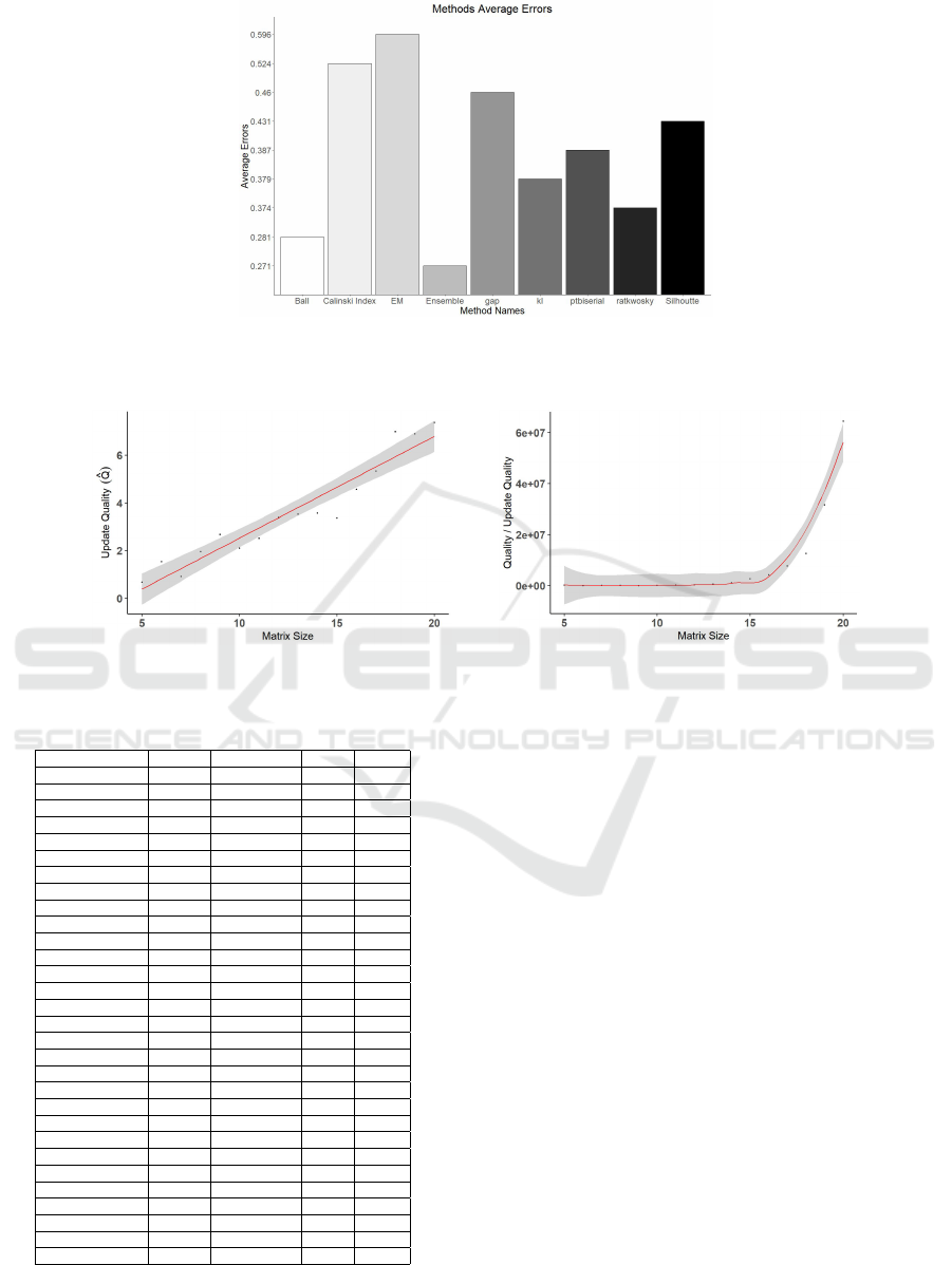
Figure 3: Normalised Average Errors on the Twenty-Eight datasets.
(a) Update Quality. (b) Update Quality Vs Exhaustive.
Figure 4: Runtime for the Quality Metrics.
Table 4: Error Values: Fair, Moderate, Median, Average.
Datasets Fair (0.4) Moderate (0.6) Median Average
aml28 0.400 0.600 0.000 0.400
Atom 2.000 2.500 3.000 3.000
BezdekIris 0.000 0.000 0.000 0.000
Blobs 0.000 0.000 0.000 0.000
Cassini 0.333 0.333 0.333 0.000
Compound 0.200 0.600 0.400 0.400
Curves1 1.000 1.333 0.000 0.000
Gaussian500 1.000 0.600 0.400 0.000
Glass 0.571 0.143 0.429 0.429
Hepta 0.143 0.000 0.571 0.571
Longsquare 0.167 0.333 0.667 0.000
Lsun 0.000 0.000 1.000 1.000
Pearl 1.333 1.333 0.667 0.667
Pmf 0.600 0.000 0.200 0.200
Shapes 0.000 0.000 0.000 0.000
Size1 0.000 0.000 0.000 0.000
Size2 0.000 0.000 0.000 0.000
Spherical˙5˙2 0.000 0.200 0.000 0.000
Square2 0.000 0.000 0.000 0.000
Synthetic control 0.000 0.000 0.167 0.000
Tetra 0.000 0.000 0.250 0.250
Tetragonular Bee 0.333 0.333 0.333 0.333
ThreeMC 0.000 0.000 0.333 0.333
Triangle1 0.000 0.000 0.000 0.000
Twosp2glob 0.500 0.000 0.000 0.000
Vehicle 0.000 0.000 0.000 0.000
Veronica 0.000 0.143 0.000 0.000
Zelnik3 1.667 0.000 0.000 0.000
0.366 0.302 0.313 0.271
Correct Estimates 10 16 10 17
6 RESULTS AND DISCUSSIONS
This paper offered methods for estimating the num-
ber of clusters in datasets using subsets from input se-
lected from binary and the Gray code. We present the
result of four groups of experiments conducted using
different thresholds of Weighted Kappa values - aver-
age, fair, moderate and median. To ascertain which
of the four values best predict the average number of
clusters in the datasets, we recorded cases where the
predictions were off and how far off the predicted re-
sults were from the number of clusters reported as er-
rors. The cumulative errors of the datasets are shown
for each case in Table 3. We equally measure the
speed difference between the Quality and the update
Quality implementations, and the results are reported
below.
6.1 Estimated Errors
We calculated the cumulative error for the datasets as
shown in equation 8 using the absolute average dif-
ference between the predicted values for each method
taken from the actual number of clusters. We used
the absolute value of the difference to normalise the
Estimating the Optimal Number of Clusters from Subsets of Ensembles
389

errors. We compared the best threshold from the en-
sembles to the earlier-mentioned methods. The error
values in table 3 show that overall the average thresh-
old predicted seventeen of the datasets correctly, fol-
lowed by sixteen for moderate, and both fair and me-
dian had ten (10) each. Similarly, the average error of
0.271 was the best for the average threshold. There-
fore, we compare the results of the other methods with
the average threshold.
Error =
|Estimate −#Clusters|
#Clusters
(8)
Table 3 shows the errors for the eight methods com-
pared with the ensemble(average). Our ensemble pre-
dicted seventeen of the twenty-eight dataset correct
against twelve predicted by the Calinski Index (CH),
the best among methods considered. Similarly, the
best error estimate among the methods considered
was Ball=0.281. Although relatively close to the en-
semble, the number of clusters predicted correctly
was just eight (8).
We examine cases where the error from the en-
semble was higher than any of the other methods.
Five datasets are mentioned here: Atom, Compound,
Glass, Lsun and Tetragonular bee, where Ball, KL,
CH, Ptbiserial, and Expectation maximisation per-
formed much better than the ensemble, and we dis-
cuss in detail two of the dataset. First, the Atom
dataset consists of two clusters in three dimensions
with a completely overlapping convex hull, by defini-
tion (Ultsch, 2004), the Atom dataset is linearly non-
separable because the first cluster entirely encloses
the second. The four ensembles performed poorly in
the number of clusters predicted correctly with an er-
ror of 3.00 compared with KL, which correctly pre-
dicted the number of clusters in Atom. However, on
average, the correctly predicted number of clusters for
KL is eight against seventeen from the average en-
semble. We intend to examine the agreement matrix
produced from the initial clustering in-depth to ascer-
tain if the shape or the unique characteristics of the
dataset contributed to the error margin. Second, the
Lsun dataset initially published in (Thrun and Ultsch,
2021) was based on the two-dimensional version of
the dataset, and the challenge is the unique character-
istics of non-overlapping convex hulls, varying geo-
metric shapes, and pockets of outliers. At the time
of this writing, we are yet to explore factors such as
differences in the shapes of the clusters, variance be-
tween the inner clusters, and cluster separations to
see how they may have contributed to the error es-
timate observed in the ensemble. In conclusion, the
four ensemble technique’s error is less on average
for all datasets. Second, the number of datasets cor-
rectly estimated compared with the actual clusters in
the datasets also confirms that the clustering ensem-
ble is a preferred alternative to all the other methods
considered.
6.2 Quality vs Update Quality
The update quality uses the previous subset qual-
ity value to calculate the next quality. It compares
the pairs of the subset (the unique pairs) for differ-
ence, and depending on the difference in combina-
tion; the next subset quality is calculated as an update
ˆ
Q by adding or subtracting based on the difference,
as shown in equation 7. Using previous values of the
quality in calculating the next quality improves the
calculation of the subsequent subset’s quality and re-
duces the number of iterations. We measure the per-
formance of the quality and update quality on sim-
ulated data. The data consists of a symmetric ma-
trix using the R program’s random uniform distribu-
tion from intervals 0.1 and 0.97 (intervals could be
from any range) — the symmetric matrix range from
5...20, which corresponds to the number of input clus-
terings. The result, as expected, shows that the update
quality implementation performs better than the orig-
inal quality function, as shown in Figure 4. The result
confirms the earlier theoretical framework in runtime
improvement.
7 CONCLUSION AND FUTURE
WORK
This paper introduces a novel ensemble technique that
uses subsets of ensembles to estimate the number of
clusters in the dataset. Compared to similar methods,
the method’s performance shows that our approach is
promising, both in the number of clusters correctly
predicted and the error in the prediction, as demon-
strated in the outputs above. We envisage that speed
will be a problem as the number of datasets and in-
put methods increases. The Gray code version re-
duces the runtime from quadratic to linear time. How-
ever, the approach may no longer be feasible as the
input size grows. It would be interesting to explore
whether a heuristic search approach could speed up
the method in future implementations.
REFERENCES
Arica, N. and Yarman-Vural, F. T. (2001). An overview
of character recognition focused on off-line handwrit-
ing. IEEE Transactions on Systems, Man, and Cyber-
DATA 2022 - 11th International Conference on Data Science, Technology and Applications
390

netics, Part C (Applications and Reviews), 31(2):216–
233.
Ayed, S., Arzoky, M., Swift, S., Counsell, S., and Tucker, A.
(2018). An exploratory study of the inputs for ensem-
ble clustering technique as a subset selection problem.
In Proceedings of SAI Intelligent Systems Conference,
pages 1041–1055. Springer.
Ball, G. H. and Hall, D. J. (1965). Isodata, a novel method
of data analysis and pattern classification. Technical
report, Stanford research inst Menlo Park CA.
Calinski, R. and Harabasz, G. (1974). A dendrite method
for cluster analysis. Communications in Statistics,
pages 1–27.
Charrad, M., Ghazzali, N., Boiteau, V., and Niknafs, A.
(2014). Determining the number of clusters using
nbclust package. MSDM, 2014:1.
Doran, R. W. (2007). The gray code. J. Univers. Comput.
Sci., 13(11):1573–1597.
Dua, D. and Graff, C. (2017). Uci machine learning reposi-
tory.
Fern, X. Z. and Brodley, C. E. (2004). Solving cluster en-
semble problems by bipartite graph partitioning. In
Proceedings of the twenty-first international confer-
ence on Machine learning, page 36. ACM.
Fr
¨
anti, P. and Sieranoja, S. (2018). K-means properties on
six clustering benchmark datasets.
Giacinto, G. and Roli, F. (2001). Design of effective neural
network ensembles for image classification purposes.
Image and Vision Computing, 19(9-10):699–707.
Hamerly, G. and Elkan, C. (2003). Learning the k in k-
means. Advances in neural information processing
systems, 16.
Higham, D. J., Kalna, G., and Kibble, M. (2007). Spectral
clustering and its use in bioinformatics. Journal of
computational and applied mathematics, 204(1):25–
37.
Hubert, L. and Arabie, P. (1985). Comparing partitions.
Journal of classification, 2(1):193–218.
Jain, A. K., Murty, M. N., and Flynn, P. J. (1999). Data
clustering: a review. ACM computing surveys (CSUR),
31(3):264–323.
Kass, R. E. and Wasserman, L. (1995). A reference
bayesian test for nested hypotheses and its relation-
ship to the schwarz criterion. Journal of the american
statistical association, 90(431):928–934.
Kent, J., Bibby, J., and Mardia, K. (2006). Multivariate
analysis (probability and mathematical statistics).
Krzanowski, W. J. and Lai, Y. (1988). A criterion for deter-
mining the number of groups in a data set using sum-
of-squares clustering. Biometrics, pages 23–34.
Li, T., Ding, C., and Jordan, M. I. (2007). Solving con-
sensus and semi-supervised clustering problems using
nonnegative matrix factorization. In Seventh IEEE
International Conference on Data Mining (ICDM
2007), pages 577–582. IEEE.
Milligan, G. W. (1981). A monte carlo study of thirty inter-
nal criterion measures for cluster analysis. Psychome-
trika, 46(2):187–199.
Pelleg, D., Moore, A. W., et al. (2000). X-means: Extend-
ing k-means with efficient estimation of the number of
clusters. In Icml, volume 1, pages 727–734.
Ratkowsky, D. and Lance, G. (1978). Criterion for deter-
mining the number of groups in a classification. Aus-
tralian Computer Journal.
Rayana, S. (2016). ODDS library.
Rousseeuw, P. J. (1987). Silhouettes: a graphical aid to
the interpretation and validation of cluster analysis.
Journal of computational and applied mathematics,
20:53–65.
Strehl, A. and Ghosh, J. (2002). Cluster ensembles—
a knowledge reuse framework for combining multi-
ple partitions. Journal of machine learning research,
3(Dec):583–617.
Sugar, C. A. and James, G. M. (2003). Finding the num-
ber of clusters in a dataset: An information-theoretic
approach. Journal of the American Statistical Associ-
ation, 98(463):750–763.
Swift, S., Tucker, A., Crampton, J., and Garway-Heath, D.
(2007). An improved restricted growth function ge-
netic algorithm for the consensus clustering of reti-
nal nerve fibre data. In Proceedings of the 9th annual
conference on Genetic and evolutionary computation,
pages 2174–2181. ACM.
Swift, S., Tucker, A., Vinciotti, V., Martin, N., Orengo, C.,
Liu, X., and Kellam, P. (2004). Consensus clustering
and functional interpretation of gene-expression data.
Genome biology, 5(11):1–16.
Thrun, M. C. and Ultsch, A. (2021). Swarm intelligence
for self-organized clustering. Artificial Intelligence,
290:103237.
Ultsch, A. (2004). Strategies for an artificial life system to
cluster high dimensional data. Abstracting and Syn-
thesizing the Principles of Living Systems, GWAL-6,
pages 128–137.
Vishnuvarthanan, G., Rajasekaran, M. P., Subbaraj, P., and
Vishnuvarthanan, A. (2016). An unsupervised learn-
ing method with a clustering approach for tumor iden-
tification and tissue segmentation in magnetic reso-
nance brain images. Applied Soft Computing, 38:190–
212.
West, D., Dellana, S., and Qian, J. (2005). Neu-
ral network ensemble strategies for financial deci-
sion applications. Computers & operations research,
32(10):2543–2559.
Zhang, Y. and Zhao, Y. (2004). Automated clustering algo-
rithms for classification of astronomical objects. As-
tronomy & Astrophysics, 422(3):1113–1121.
Estimating the Optimal Number of Clusters from Subsets of Ensembles
391
