
Calibration of the Nonlinear Wheel Odometry Model with an Improved
Genetic Algorithm Architecture
M
´
at
´
e Fazekas, Bal
´
azs N
´
emeth and P
´
eter G
´
asp
´
ar
Institute for Computer Science and Control, SZTAKI-ELKH, Kende u. 13-17., Budapest, Hungary
Keywords:
Parameter Estimation, Nonlinear Model, Genetic Algorithm.
Abstract:
To guarantee the required motion estimation accuracy for an autonomous vehicle, the integration of the wheel
encoder measurements is an adequate choice besides the generally applied GNSS, inertial and visual-odometry
methods. Wheel odometry is a robust and cost-effective technique, but the required calibration of the nonlinear
odometry model in the presence of noise remains an open problem in the context of autonomous vehicles. The
core problem is that due to the nonlinear behavior of the model, the identified parameters will be biased even
with Gaussian-type measurement noises. The presented method operates with genetic algorithms and utilizes
two novel improvements: compensation of the state initialization of the model inside the estimation process,
and equilibration of the parameter estimation by an adaptive weighting technique. With these innovations
the distortion effects are mitigated and unbiased model calibration can be obtained even when several local
minimums exist. The performance of the developed algorithm and the accuracy of parameter estimation are
demonstrated with detailed validation and test with a real vehicle.
1 INTRODUCTION
The state estimation has a critical responsibility in the
self-driving software because the trajectory planning
and motion control are based on its results. The aim is
to determine the motion signals, such as velocities and
pose (position and orientation) as accurately as possi-
ble, and the robust estimation is also a required capac-
ity in parallel. However, cost-efficiency is important
in the automotive industry as well, thus the applied
automotive-grade type sensors are from the low-cost
ones. The disadvantages of the GNSS (Global Navi-
gation Satellite System), IMU (Inertial Measurement
Unit), or vision-based methods can be improved with
the integration of the wheel encoder measurements
(Funk et al., 2017). Nevertheless, the model contain-
ing the encoder measurements suffers from parameter
uncertainty. Therefore, this paper focuses on the cal-
ibration of the odometry model which is equivalent
to the parameter estimation of a nonlinear dynamic
system. This type of optimization task behind the
calibration process is not solved yet in general, see
e.g. (Schoukens and Ljung, 2019), and the problem
is more difficult if noisy measurements are applied,
such as IMU, GNSS, and wheel-encoder signals.
Most of the related works in the field of odometry
calibration deal with mobile robots. A widely applied
method is the Augmented Kalman-filter (Martinelli
and Siegwart, 2006; Brunker et al., 2017), in which
the parameters are estimated simultaneously with the
state filtering. Although the solution is simple, ob-
servability issue, convergence difficulty, and unstable
behavior can appear, see (Antonelli and Chiaverini,
2007), (Censi et al., 2013).
The other way is to estimate the parameters in a re-
gression task. However, due to the nonlinear model,
the optimization leads to a non-convex problem that
is difficult to solve. Separation, or double lineariza-
tion are applied in some works (Antonelli et al., 2005;
Censi et al., 2013; Seegmiller et al., 2013), to simplify
the nonlinear calibration task. Nevertheless, these can
be only applied with simple and separable models,
but for the proper modeling of the behavior of a real-
sized car an improved odometry model is necessary
(Fazekas et al., 2020).
From the identification scope issues, which even
not appear at all in the case of linear system identifi-
cation (Ljung, 1987), are revealed from the theoretical
point of view (Schoukens and Ljung, 2019). Since the
model is nonlinear, linearization and a recursive esti-
mation are necessary (Tangirala, 2015). In this case,
the initial states of the dynamic model have to be ini-
tialized with measurements containing noise, which
introduces a new problem. The noise is affected by
640
Fazekas, M., Németh, B. and Gáspár, P.
Calibration of the Nonlinear Wheel Odometry Model with an Improved Genetic Algorithm Architecture.
DOI: 10.5220/0011275700003271
In Proceedings of the 19th International Conference on Informatics in Control, Automation and Robotics (ICINCO 2022), pages 640-648
ISBN: 978-989-758-585-2; ISSN: 2184-2809
Copyright
c
2022 by SCITEPRESS – Science and Technology Publications, Lda. All rights reserved

the nonlinearity, thus its effect on the measured out-
put is no longer familiar with the Gaussian frame-
work, which is applied in almost all methods, such
as Kalman-filtering, least squares etc (Ljung, 2010).
Thus, the parameter estimation will be certainly bi-
ased. Other methods, such as genetic algorithm, that
apply random sampling and heuristic based improve-
ments for the convergence instead the gradient, can
be used as well, but the distortion effect due to the
initialization noise also appears.
The available measurements for the model cali-
bration and the compensation of the noises are al-
ways crucial questions. In several papers, a restric-
tive requirement is applied, e.g. special pre-defined
paths for the vehicle (Jung et al., 2016), unbiased es-
timation of the initial pose (Antonelli et al., 2005),
or measurements with expensive sensors (Censi et al.,
2013). To the best of our knowledge, (Maye et al.,
2016) is the only paper that deals with the distortion
effect of the noises in the odometry parameter esti-
mation, but with a special focus on the observability.
If more measurements are available, the optimization
can be performed in a batch mode to reduce the im-
pact of the initialization noise, however, a weighting
is recommended (Seegmiller et al., 2013).
This work focuses on the compensation of the ini-
tial state noises, and the determination of the relative
weights between segments forming a batch. Measure-
ments only from cost-effective automotive-grade type
sensors, such as GNSS, IMU, compass and wheel en-
coders are utilized, and the signals are saved on real
streets. In the proposed algorithm the initial states
are handled as parameters, and the estimation is per-
formed with genetic algorithms in a complex archi-
tecture. The main contribution is that the proposed
method transforms the fully explored parameter space
by the genetic algorithm into an adaptive weighting
procedure. The efficiency of the proposed algorithm
is validated with experimental tests of a real-sized ve-
hicle, which demonstrates that the mentioned issues
of the noises can be mitigated, and the estimation ac-
curacy can be significantly improved.
The remainder of the paper is organized as fol-
lows. In Section 2, the applied odometry model is
presented which includes dynamic effects in order to
ensure a proper model for the calibration. Next, the
Section 3 introduces the issues of the nonlinear model
calibration and summarizes the estimation with a ge-
netic algorithm. The proposed architecture for the cal-
ibration can be found in Section 4. The measurement
scenarios applied for the estimation are presented in
Section 5.1. The validity of our approach is demon-
strated via vehicle test experiments in Section 5, and
finally, the paper is concluded in Section 6.
a
y
: lateral acceleration
(measured)
β: sideslip angle
(filtered)
n
rl/rr
: wheel rotation
(measured)
Figure 1: Odometry model.
2 VEHICLE MODEL
The navigation with wheel odometry is based on a
model, where the state vector x
t
contains the pose,
the longitudinal and lateral positions of the center of
gravity p
x,t
, p
y,t
, and the ψ
t
orientation of the vehicle.
The change of the pose is based on the longitudinal
v
t
and angular ω
t
velocities, thus the planar motion of
the vehicle in t discrete time steps is calculated as,
p
x,t+1
p
y,t+1
ψ
t+1
=
p
x,t
+ v
t
· T
s
· cos(ψ
t
+ ω
t
/2 · T
s
+ β
t
)
p
y,t
+ v
t
· T
s
· sin(ψ
t
+ ω
t
/2 · T
s
+ β
t
)
ψ
t
+ ω
t
· T
s
,
(1)
where β
t
is the filtered sideslip angle. The velocities
are computed utilizing the n wheel rotations,
v
t
= (n
rl,t
· c
rl,t
+ n
rr,t
· c
rr,t
)/2, (2a)
ω
t
= (n
rr,t
· c
rr,t
− n
rl,t
· c
rl,t
)/t
r
, (2b)
where T
s
= 0.025 s is the sampling time, c
rl,t
,c
rr,t
are
the actual wheel circumferences, and t
r
is the rear
track width. In the literature, the slight change of the
wheel radius due to the effect of vertical dynamic is
generally neglected, because the odometry-based lo-
calization is widely used in low-speed circumstances,
e.g., automated parking. However, our method is de-
veloped for general driving, where the dynamics is
significant (Fazekas et al., 2020). Therefore, the slight
change due to the vertical load transfer is considered,
c
rl,t
= c
e
+ c
d
/2 + d · a
y,t
, (3a)
c
rr,t
= c
e
− c
d
/2 − d · a
y,t
, (3b)
where the c
e
is the effective wheel circumference, c
d
is the difference between the effective values, a
y,t
is
the lateral acceleration measured by the IMU, and the
dynamic component d takes into account the effect of
vertical dynamics.
In the calibration process, every state variable is
measured, thus the system model is,
x
t+1
= f (x
t
,u
t
,θ), x
t
= [p
x,t
, p
y,t
,ψ
t
]
T
, y
t
= x
t
,
(4a)
u
t
= [n
rl,t
,n
rr,t
,β
t
,a
y,t
]
T
, θ = [c
e
,c
d
,t
r
,d], (4b)
where f (·) contains (1), and θ is the parameter vector.
The values are illustrated in the paper with the units
Calibration of the Nonlinear Wheel Odometry Model with an Improved Genetic Algorithm Architecture
641

of m, mm,m,mm · s
2
/m for the c
e
,c
d
,t
r
,d parameters,
respectively.
The nominal values of c
e
and t
r
can be found in
the vehicle datasheet, but with these values the posi-
tion error is already in the range of 10 m after a few
hundred meters. Moreover, the c
d
and d parameters
are unknown, thus the calibration is essential.
3 CALIBRATION OF
NONLINEAR MODELS
3.1 General Methods
The calibration problem of a physical model contains
the estimation of system parameters Θ, which leads to
an optimization task. Generally, this is formulated as
a minimization problem of the squared errors of the
output, such as
ˆ
Θ
opt
= arg min
Θ
V
K
(Θ) = arg min
Θ
K
∑
k=1
||
e
y
k
− ˆy
k
(Θ)||
2
,
(5)
where the ˆy
k
(Θ) is the predictor of the model,
ˆy
k
(Θ) = h(x
k
) x
k+1
= f (x
k
,
e
u
k
,Θ), (6)
and
e
u
k
−
e
y
k
are measured input-output signals. The
methods to solve (5) can be grouped according to the
usage of gradient techniques.
In the one group, the optimization is solved with
the well-known least squares (LS) method which ap-
plies the gradient directly. However, in the case of
nonlinear models, the dynamic system can not be or-
dered into the basic least squares form as ˆy
k
(Θ) =
φ
T
k
(
e
u
k
)Θ, see (Ljung, 1994). Therefore numerical
search is required (Tangirala, 2015), where the Gauss-
Newton approach is an adequate choice. In this case,
the nonlinear least squares problem is handled with
the Taylor-approximation of the predictor forming a
locally linear estimation and an iterative solution.
The other group contains methods that do not use
any gradient to solve the minimization, e.g., parti-
cle filter or genetic algorithm. Instead, random sam-
pling of the parameter space, evaluation with the mea-
sured input-output signals, and heuristic-based im-
provements of the possible solutions are applied to
reach the optimum.
3.2 Core Problem of Nonlinear
Dynamic Model Calibration
Regardless of the applied methods, the calibration of
a nonlinear dynamic model has a core problem. The
outputs of system model (6) have to be computed with
the actual parameter values which requires the initial-
ization of the states x
0
at the beginning of the estima-
tion window. In the odometry model, the output is
equal with the state (y
k
= x
k
), thus the measured
e
y
k=0
can be utilized for the initialization,
b
y
1
(Θ)
.
.
.
b
y
K
(Θ)
=
x
1
.
.
.
x
K
=
f (x
0
,
e
u
0
,Θ)
.
.
.
f (x
K−1
,
e
u
K−1
,Θ)
| x
0
=
e
y
0
.
(7)
Due to the appeared noise on it, the integrated model
diverges from the correct path even with the true pa-
rameter values. Thus, without proper initialization the
parameter estimation is biased, because the optimum
of (5) differs from the true value of Θ.
3.3 Estimation in Batch Formulation
The distortion effect of state initialization can be han-
dled, if more K long measurement segments are ap-
plied at once, such as
ˆ
Θ
opt
= arg min
Θ
N
∑
n=1
K
∑
k=1
||
e
y
n,k
− ˆy
n,k
(Θ)||
2
, (8)
where N denotes the batch size. For example, in the
case of Gauss-Newton method the Jacobian matrices
of the segments are stacked into a huge matrix and the
parameters are identified in the same iterative way, or
in the sampling based methods the actual parameter
values are evaluated for all of the N segments.
Since the model fitting is performed to every seg-
ment simultaneously, the bias resulted by the uncer-
tain state initialization is mitigated. The method can
be interpreted as a cross-validation technique inside
the estimation process, but it will be illustrated that
the optimum of the batch is not necessarily identical
with the true value of the parameters. Furthermore, a
new issue arises with the batch formulation. The seg-
ments are differs in shape of the path, velocity, or the
appearing noise of the initialization etc. Therefore,
the segment with the highest error has more influence
on the optimum, which is unfavourable. Thus, rela-
tive weighting between the segments are requested to
be introduced to equilibrate the optimization to obtain
the true value of the parameters.
3.4 Initial State as Parameter
The distortion effect of the inaccurate state initializa-
tion can be eliminated, if the poses at the beginning
of the segments are estimated as well (Fazekas et al.,
2021). In our algorithm the initial state, when the
ICINCO 2022 - 19th International Conference on Informatics in Control, Automation and Robotics
642
model outputs are calculated in (7), is included as a
parameter to be estimated, such as
x
1
= f (ϑ,
e
u
0
,Θ), ϑ = x
0
= [p
x,0
, p
y,0
,ψ
0
]
T
. (9)
In the paper, the θ contains the vehicle parameters
(4b), ϑ is the state initialization parameters (9), and
Θ denotes the parameters to be estimated, specifying
at the actual method how to include θ and ϑ.
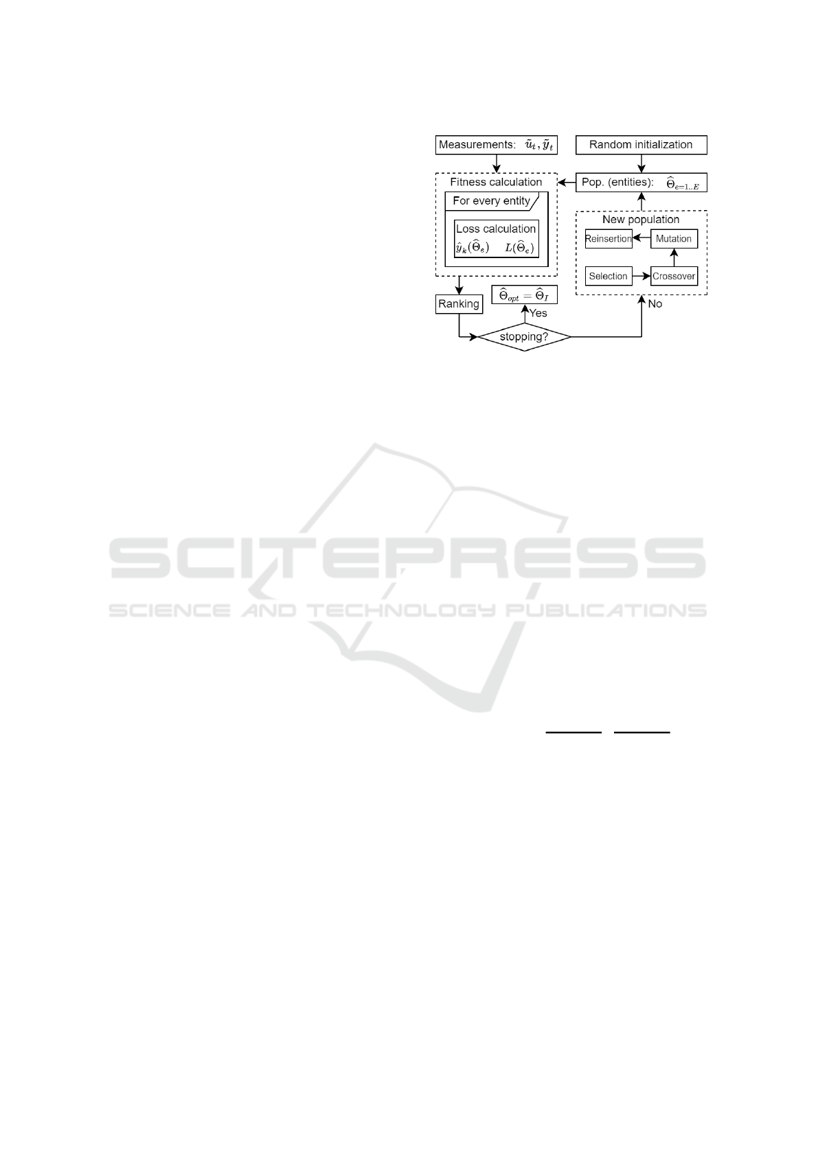
3.5 Parameter Estimation with Genetic
Algorithms
When the optimization problem of (5) has several lo-
cal optimums, the genetic algorithm (GA) is a proper
choice, because this procedure explores the entire pa-
rameter space. The estimation process is illustrated in
Figure 2. The method starts with the initialization of
E pieces of entities (model settings) by random sam-
pling, but only from a given range around the nominal
values of the estimated parameters. Next, the popula-
tion is tested, where the outputs of the model param-
eterized with the entities are calculated. The entities
are ranked by the loss, and if the stopping condition
does not occur, a new population is generated. The
main idea of the GA is to apply genetic operators or
functions inspired by the process of natural selection
to obtain convergence to the global optimum.
We use the implemented version of GA in MAT-
LAB (Mathworks, 2021a), which is based on (Gold-
berg, 1989). The Selection function chooses the enti-
ties as parents to form the new generation of the pop-
ulation. The mathematical method is the stochastic
universal sampling (Baker, 1987). These are paired
(
b
Θ
a
,
b
Θ
b
), and the new entities are calculated with the
Crossover function, such as
b
Θ
new
=
b
Θ
α
+ ξ · (
b
Θ
β
−
b
Θ
α
), (10)
where ξ is a vector containing random numbers from
the range [0,1]. The Mutation function enables the
GA to search further away from the actual entities.
With a low probability (5%), when the crossing is ex-
ecuted a random vector is added to the ξ, which helps
to avoid sticking into a local optimum. The final step
of the formulation of the new population is the Rein-
sertion. The stable convergence is ensured with the
so-called ”elite strategy”, where the best entities (5%
in our case) in the current generation are guaranteed
to survive to the next generation. The other entities
are chosen based on the loss values, the best 95% of
the entities from the current population and the newly
generated 0.8E ones with the crossover and mutation
are collected. This iterative evolution of the popula-
tion continues until the stopping condition, e.g. max-
imum generation or lower improvement of the best
entity than a given limit, is reached.
Figure 2: Process of the GA based estimation.
4 PROPOSED ARCHITECTURE
4.1 Parameter Estimation with
Initialization Compensation
The θ vehicle parameters are identified in batch mode
with N segments, where the initial state of every seg-
ment are also estimated. Since a ϑ
n
initialization
value is independent from the other segments in the
batch, several local minimums are exist. Therefore,
in our method, the GA is applied for the optimiza-
tion, because this procedure uses random sampling,
making it a suitable methodology for solving prob-
lems with several local minimums.
The parameter vector and the cost function is the
following,
b
Θ = [
b
θ,
b
ϑ
1
,...
b
ϑ
N
]
T
, (11a)
b
Θ
opt
= arg min
b
Θ
N
∑
n=1
K
∑
k=1
l(
e
y
n,k
,
b
y
n,k
(
b
θ,
b
ϑ
n
),W
n
)
| {z }
L
n
, (11b)
l(·) =
h
e
y
n,k
−
b
y
n,k
(
b
θ,
b
ϑ
n
)
i
T
W
n
h
e
y
n,k
−
b
y
n,k
(
b
θ,
b
ϑ
n
)
i
,
(11c)
where L
n
is the loss of a segment, and W
n
is a weight
matrix which is formulated, such as
W
n
= w
r,n
· diag([w
p,x
,w
p,y
,w
ψ
]
T
1x3
). (12a)
The w
p,x
,w
p,y
,w
ψ
are the weights of the system equa-
tions (4) to compensate the different magnitude of the
position error in meter and orientation error in radian,
and thus these are the same for every segment in the
batch. The values are determined with an experimen-
tal tuning, the optimal setting is resulted as
[w
p,x
,w
p,y
,w
ψ
] = [1,1,40], (13)
Calibration of the Nonlinear Wheel Odometry Model with an Improved Genetic Algorithm Architecture
643
because only the ratio of the weights matters. In con-
trast, the w
r,n
is the relative weight between the seg-
ments to prevent that some segments has higher influ-
ence than others on the estimated vehicle parameters.
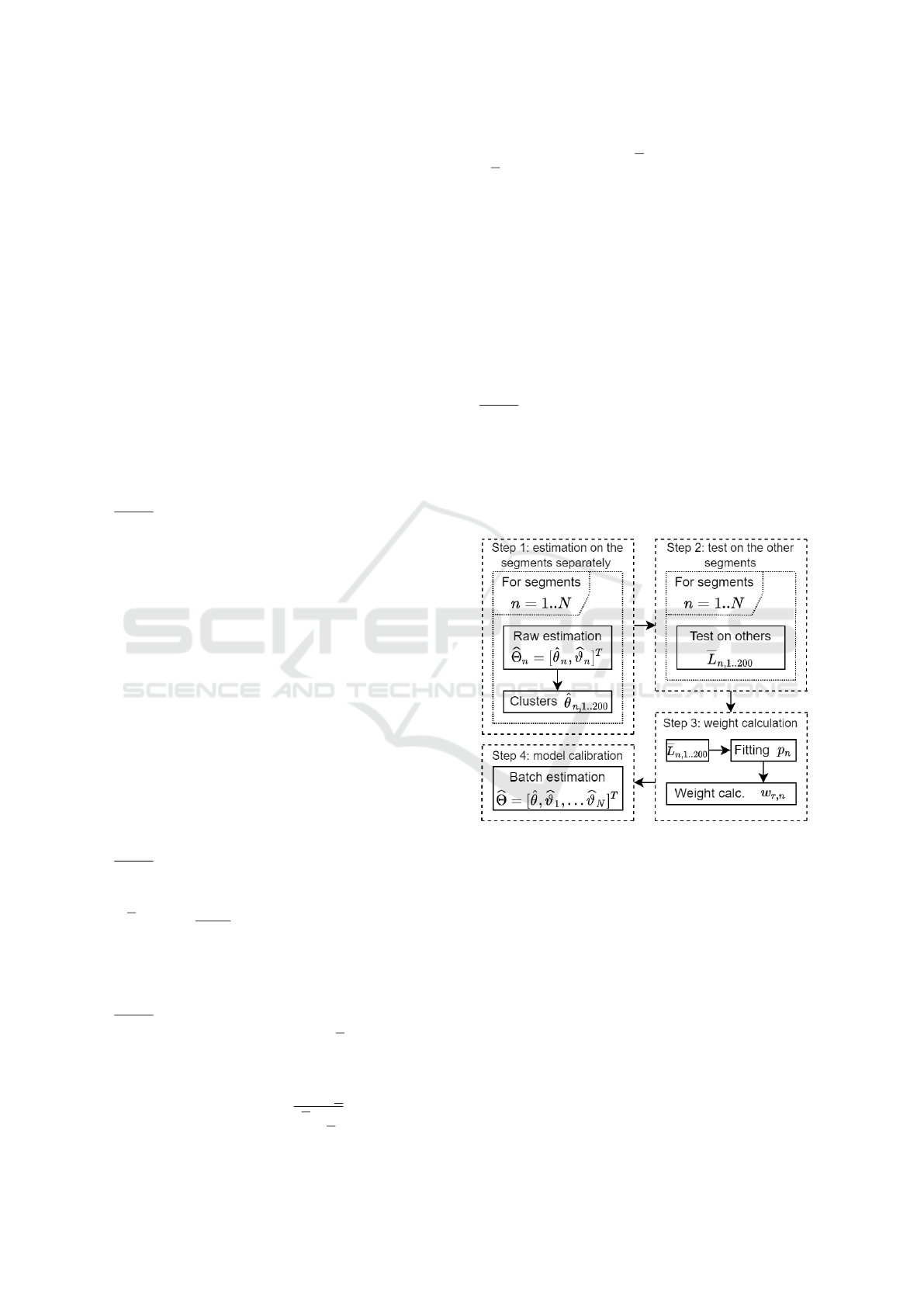
4.2 Architecture with Relative
Weighting
Our proposed method integrates a cross-validation
based knowledge to determine the proper relative
weight of the segments. The main idea is that a seg-
ment whose optimal model setting (which minimizes
the L
n
individual segment error) has a high error on
the other segment of the batch should not have signif-
icant weight in the parameter identification. This idea
is implemented in the architecture presented in Fig-
ure 3, where there are 3 steps to determine the proper
w
r,n
weights, before the model is calibrated with the
presented method in the previous section.
Step 1: In the first step, GA based estimation is per-
formed on the segments separately (raw mode). In
this step, i
max
= 7 generations are applied with a pop-
ulation size of E = 2000. Because most of the odom-
etry parameters are geometry ones, the search space
can be constrained with the following lower- and up-
per bounds
θ
lb
= [1.93,−5,1.4,−1]
T
, θ
ub
= [1.97,5,1.7,3]
T
.
(14)
The initial state parameters are also bounded around
the corresponding
e
y
n,k=0
filtered pose value
ϑ
lb
=
e
y
n,k=0
− [3,3,0.2]
T
, ϑ
ub
=
e
y
n,k=0
+ [3,3,0.2]
T
.
(15)
Since the entire parameter space is explored dur-
ing the convergence, k-means clustering is performed
(Mathworks, 2021b). The parameter space of every
segment is represented with C = 200 clusters (
b
θ
n,1..200
sorted by the L
n
loss) formed from the last 5 genera-
tions of entities.
Step 2: In the second step, the clustered models are
tested on the other segments of the batch, and the av-
erage error is computed,
L
n,1..200
=
1
N − 1
N
∑
m=1
L
m
(
b
θ
n,1..200
,
b
ϑ
m
), (m 6= n)
(16)
where L
m
(
b
θ
n,c
,
b
ϑ
m
) is the loss on the m segment with
the c −th clustered model of the n segment.
Step 3: The mentioned cross-validation based knowl-
edge is transformed to w
r,n
relative weights in this
step. Straight line is fitted to the L
n,1..200
errors of
the segments, and the weights are calculated in the
following way,
w
r,n
= 1 + 2 ·
p
1,n
− p
p − p
, (17a)
p = min(p
1,n=1..N
)), p = max(p
1,n=1..N
)), (17b)
where p
1,n
is the steepness of the fitted straight of
segment n. This scheme determines the w
r,n
rela-
tive weights between 1 and 3, and means that the
weight of a segment, whose individual optimal set-
tings (which have increasing error on the actual seg-
ment) have decreasing error on the other ones, will be
low. In contrast, the segments, whose sorted clustered
models have similarly increasing error on the other
segments, will get higher weights. Thus, the impact
of segments that results in possible incorrect calibra-
tion can be mitigated, and in parallel, the estimation
bias should be lower.
Step 4: Finally, the odometry model is calibrated with
the GA in batch mode utilizing the pre-calculated w
r,n
weights. The bounds for the θ and ϑ parameters are
the same as in Step 1, but since in the batch mode the
number of parameters is 34 (4 vehicle, and N = 10
times 3 initial state parameters), i
max
= 10 genera-
tions with a population size of E = 10000 is utilized
to reach the global optimum.
Figure 3: Calibration architecture of the proposed method.
5 EXPERIMENTAL RESULTS
5.1 Test Measurement Scenario
The test vehicle is a Nissan Leaf electric car which
is equipped with automotive-grade GNSS, compass,
and IMU sensors, and from the vehicle CAN bus the
wheel encoder signals are also saved. The sampling
frequency is 40 Hz. The test track is a 24 km long
route in suburb and city driving under normal driv-
ing conditions. The track contains various bends, two
roundabouts, and lots of crossroads.
ICINCO 2022 - 19th International Conference on Informatics in Control, Automation and Robotics
644
The signals of the GNSS, compass, and IMU sen-
sor are utilized for the model calibration. The pose
can be measured directly with the first two, although
these signals are assumed to be noisy but unbiased. In
contrast, the pose computation from the acceleration
and angular velocity measurements with the IMU is
generally biased, but the noise is lower. The filtering
problem is well-explored, the implemented method
is similar to (Caron et al., 2006) to obtain reference
output measurements (
e
y
t
) for the calibration. The
sideslip is also estimated with an IMU-based method
(Bevly et al., 2006) in the bends, which are detected
using the vehicle trajectory.
The 24 km long route is divided into 300 m long
segments (K = 1350) with step size of 2.5 s, which re-
sults in 2037 segments. Since the c
d
,t
r
and d param-
eters can be observed properly only with the yaw rate
equations (2b), the 1127 segments with higher abso-
lute angular velocity than 0.15 rad/s are selected for
the calibration.
5.2 Validation Process and Error
The true value of the θ = [c
e
,c
d
,t
r
,d] parameters are
unknown, thus the model calibration is validated with
the position error of the resulted model. In order to
avoid overfitting, the segments are regenerated with
different initial points. Furthermore, in the validation
process, all of the segments are applied regardless of
the angular velocity is lower than the limit. The posi-
tion error of a calibrated model containing
b
θ is calcu-
lated for every segment s as,
E
p,s
=
K
∑
k=1
q
(
e
p
x,k
− p
x,k
(
b
θ))
2
+ (
e
p
y,k
− p
y,k
(
b
θ))
2
,
(18)
and the E
p
average of these are applied as a validation
error to evaluate the calibration.
Take into account that the minimum validation er-
ror is not zero, because the states of the odometry
model (4) at the beginning of the segment are ini-
tialized with the filtered pose values in the validation
process. To find the reachable minimum error, a GA-
based search has been also performed, where only the
θ vehicle parameters have been estimated. All of the
validation segments have been applied, thus it can be
an offline validation method only, but we can deter-
mine that the minimum position error in this valida-
tion case is 2.22 m.
5.3 Calibration with the Method
In this section, the calibration for a given batch with
the proposed method is illustrated step-by-step. The
detailed results demonstrate the necessity of both im-
provements as well, i.e., the integration of initial state
estimation and the relative weighting.
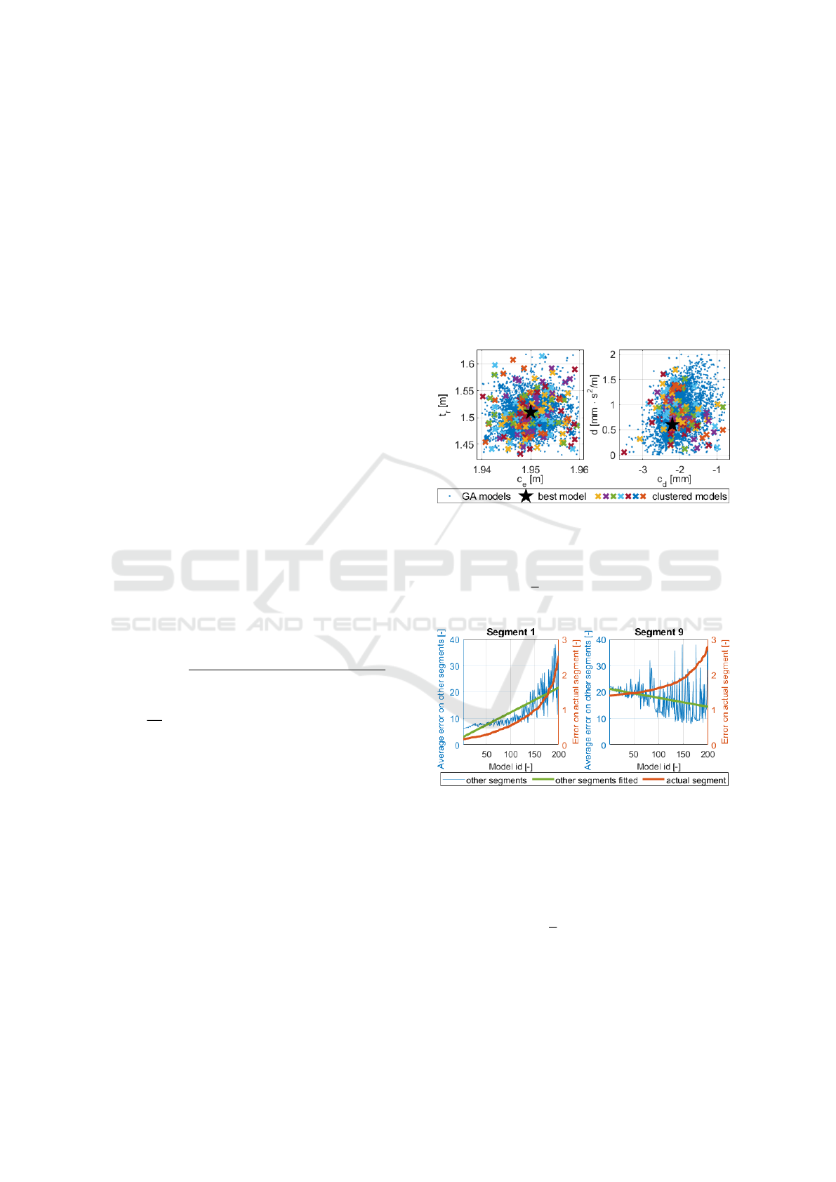
5.3.1 Segment Representation with Clusters
In Step 1, GA estimations are performed for every
segment individually. The entities of the last 5 gener-
ation of the n = 1 segment of the batch can be found
in Figure 4. Since the loss of the models are between
0.15 − 2.79, the parameters are in a wide hypercube,
e.g. the range of the t
r
track widths is 1.43 − 1.62 m.
The entities of the segment are represented with 199
Figure 4: Entities and clustered models of a segment.
clusters, which are sorted by the loss, and the best en-
tity is also used as the first ”clustered model”. In Step
2, the clustered models are tested on the other N − 1
segments and the L
n,1..200
average errors (16) are com-
puted. In Figure 5, the loss of the clustered models on
Figure 5: Errors of two segments from the batch.
the actual segment, and the average error (loss by test-
ing on others) are presented for two segments of the
batch.
5.3.2 Weight Calculation
In Step 3, the w
r,n
weights are determined. The fitted
straight lines to the L
n,1..200
average errors are illus-
trated in Figure 5 as well. For segment 1, the mod-
els with higher errors in the actual segment also have
higher errors in the other segments. In contrast, in
segment 9 it is the opposite. Thus, this segment would
Calibration of the Nonlinear Wheel Odometry Model with an Improved Genetic Algorithm Architecture
645
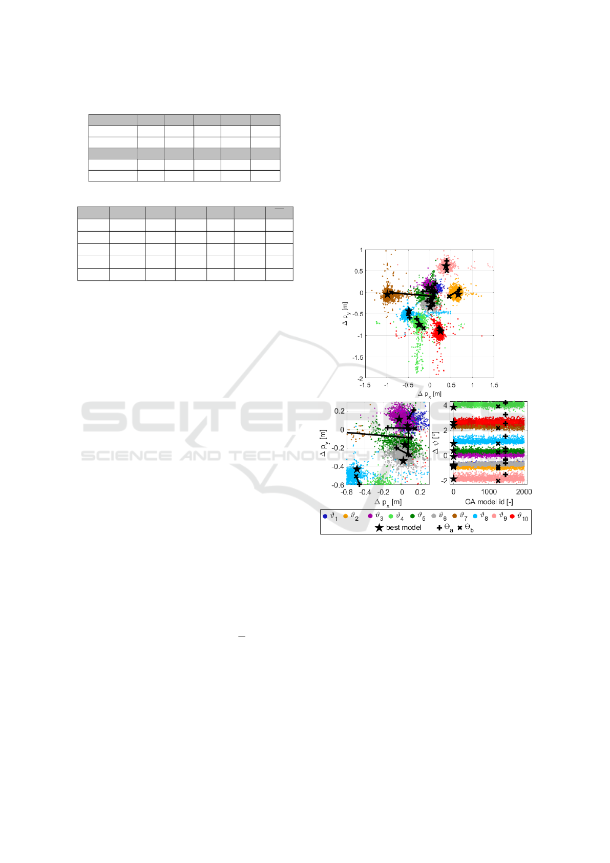
Table 1: Relative weight of the segments in the batch.
Seg. 1 2 3 4 5
p
1,n
[10
−2
] 9.41 7.55 3.65 -2.00 6.19
w
r,n
3.00 2.71 2.10 1.22 2.50
Seg. 6 7 8 9 10
p
1,n
[10
−2
] 6.94 -2.15 0.85 -3.40 -1.38
w
r,n
2.61 1.12 1.66 1.00 1.31
Table 2: Data of the best 2000 entities.
c
e
c
d
t
r
d L E
p
Min 1.9495 -2.20 1.510 0.88 0.747 2.29
Mean 1.9503 -2.08 1.517 0.93 0.758 2.37
Max 1.9513 -1.94 1.525 1.00 0.766 2.60
b
θ
a
1.9501 -1.94 1.518 0.88 0.758 2.58
b
θ
b
1.9502 -2.20 1.513 1.00 0.756 2.33
distort a good optimum of the batch, since the goal is
the minimization of the error.
The determined relative weights of the segments
with the introduced rule (17) are summarized in Table
1. These are difficult to evaluate alone, but can be
done with the examination of the individual optimal
parameters of the segments (the first ”clusters” of the
200) in Figure 7.
The segments 4,7, 9, 10 have the undesirable negative
steepness, and the optimal parameters of these seg-
ments are the most different from the batch estimated
ones, especially for the c
d
circumference difference
(Figure 7).
5.3.3 Parameter Estimation with Initialization
Compensation
In Step 4, the vehicle parameters are estimated in
batch mode in parallel with the initial states (Θ =
[θ,ϑ
1..N
]) minimizing the loss function (11). It has
been mentioned that by integrating the initial states
as parameters, the estimation in batch mode is more
complicated because a lot of local optimums exist as
the ϑ values could compensate each other.
This is demonstrated with the best 2000 entities
of the final generation of the GA based estimation.
The loss of each of these entities are between 0.747−
0.766 which is a very narrow range. The θ vehicle
parameters are in a hypercube with limits that can be
found in the first three rows of Table 2. This seems
to be a narrow parameter space, but the E
p
validation
error of each of these models are in a range of 2.29 −
2.60 m, which is a significant deviation with respect
to the minimum error of 2.22 m. This illustrates the
high parameter sensitivity of the odometry model as
well.
The reason is, although the loss is similar, the
b
ϑ
n
values of the entities are spread over a wide range
resulting in several local minimums. The estimated
state initialization parameters (the ∆ deviation from
the measured
e
y
k
for better view) of the 2000 entities
are shown in Figure 6. The average of the differences
between the maximum and minimum of the ∆p
x/y
po-
sitions, and ∆ψ orientation deviations of the N = 10
segments are 1.31 m, 1.28 m and 1.25
◦
, respectively.
This illustrates that it is possible to reach the same
loss with a wide range of estimated
b
ϑ
n
initial states,
due to the mentioned compensation property of the
initialization values. The averages of the standard de-
viations of the segments are also significant with 9.8,
and 10.2 cm for the ∆p
x/y
values.
Figure 6: Estimated initial state parameters of the entities.
For example, two entities that have almost the
same loss could have completely different estimated
initialization, as it is illustrated in Figure 6 with Θ
a
and Θ
b
. Moreover, the corresponding θ vehicle pa-
rameters can lie on the other borders of the parameter
hypercube formed by the 2000 entities as it is shown
in the last rows of Table 2. Thus, the validation er-
ror of the two resulting models are differ significantly
(2.58 m vs 2.33 m), but the almost same loss makes it
very difficult to infer this during the calibration. This
example demonstrates the difficult mathematical op-
timization generated by the integration of the initial
states as parameter and batch estimation mode. How-
ever, the genetic algorithm is able to handle this opti-
mization with many local minimums if a sufficiently
ICINCO 2022 - 19th International Conference on Informatics in Control, Automation and Robotics
646
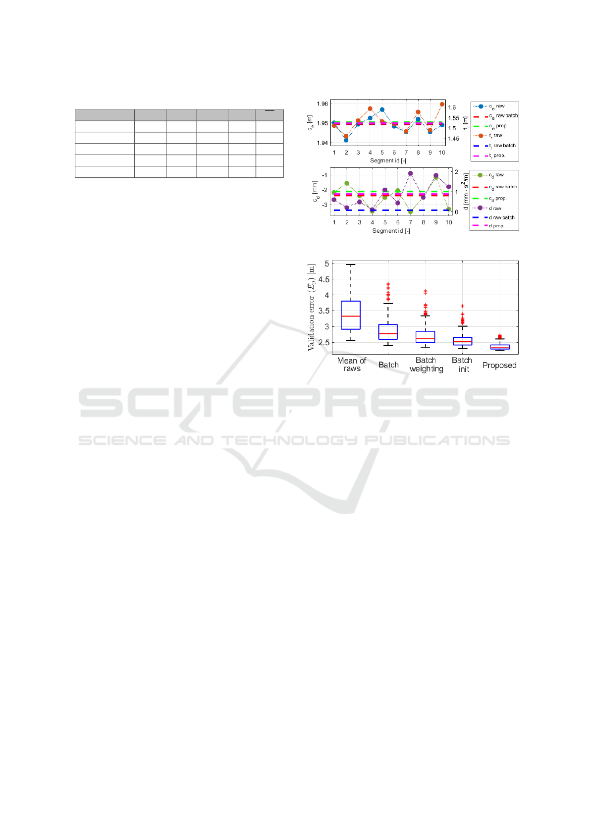
Table 3: Model calibrations of the batch with the methods.
Case c
e
c
d
t
r
d E
p
Mean of raws 1.948 -2.49 1.530 0.85 2.78
Batch 1.949 -2.40 1.519 0.07 3.97
Batch weight. 1.949 -2.27 1.525 0.07 3.50
Batch init 1.951 -2.35 1.525 1.02 2.59
Proposed 1.950 -2.13 1.523 0.87 2.29
large population is applied to explore the entire pa-
rameter space.
5.3.4 Calibration Results
In Table 3, the estimated parameters with the pro-
posed method are presented, and calibration results in
4 other cases are illustrated as well: the mean of the
results of the 10 segment with GA estimations sepa-
rately (mean of raws), identified parameters in batch
mode without any improvement (batch), with the rel-
ative weighting structure in batch mode without ini-
tialization estimation (batch weighting), and with the
estimation including the initialization parameters but
without relative weighting (batch init).
It is an interesting result that the model with the
mean of the individual (raw) GA estimations has a
lower validation error, than the batch calibrated one.
The higher error of the batch model is the conse-
quence of the widely different individual loss of the
segments, e.g. the loss of segment 4 is 12, while the
segments 1,3,5,6 have lower than 1. Therefore, the
estimated optimal parameters of the batch have to be
much closer to the individual optimum of the segment
with high loss. This is why the relative weighting
technique has been introduced.
The relative weighting technique can compensate
for this distortion a bit (third row), and when the ini-
tial parameters are taken into account this unfavorable
distortion effect is greatly reduced (fourth row). How-
ever, it is impossible to decide beforehand whether a
segment with high loss is completely wrong or only
the state initialization is highly inappropriate. There-
fore, the integration of both improvements is neces-
sary, and as we can see the validation error is further
decreased with the proposed method, which indicates
the unbiased calibration.
5.4 Results of Other Batches
In the previous section, the estimation process with
the proposed method is presented in detail on a given
batch. The robustness of the method is tested with
the formulation of 200 different batch from the 1127
segments, and the proposed calibration is performed
one by one. Only the validation errors of the batch
calibrations are presented with box-plots in Figure 8.
Figure 7: Estimated parameters with the method.
Figure 8: Validation errors of several batches.
The tests illustrate that with the batch formula-
tion the distortion effects can be mitigated, the me-
dian of the validation errors decreases to 2.77 m, from
the 3.32 m which can be reached with the mean of
the individual GA estimations of the segments. The
standard deviation is also lower with 20 cm from the
56 cm with the mean models, but the parameter es-
timation remains significantly biased. With the ap-
plication of the relative weighting method and with
the integration of the initial states as a parameter, the
errors and their standard deviations are further de-
creased, but not substantially. However, with the pro-
posed method when both improvements are applied,
the errors are in a range of 2.24 − 2.70 m, the median
error is only 2.34 m, and the 75th percentile model
has 2.42 m validation error. The standard deviation of
the errors is relatively low with 11 cm.
6 CONCLUSION
In this paper, a novel algorithm was presented for
the calibration task of the nonlinear wheel odome-
try model of an autonomous vehicle. The proposed
method introduces two innovations, the integration of
the initial state of the measurement segments as a pa-
rameter to be estimated, and a relative weighting in
Calibration of the Nonlinear Wheel Odometry Model with an Improved Genetic Algorithm Architecture
647

the batch estimation mode. The method was validated
by experimental tests with a real vehicle. The main
contribution is that when both improvements are ap-
plied, the calibration accuracy is improved.
Finally, the authors consider that with the develop-
ment of a more complex weighting, the bias-free cal-
ibration of every batch can be obtained. In the future
we would like to integrate a learning-based weight-
ing, however, the generation of training data is com-
plicated, since it is an open question what would be
the optimal weights that result in the true value of the
parameters.
ACKNOWLEDGEMENTS
The research was supported by the Ministry of Inno-
vation and Technology NRDI Office within the frame-
work of the Autonomous Systems National Labora-
tory Program. The paper was partially funded by the
National Research, Development and Innovation Of-
fice (NKFIH) under OTKA Grant Agreement No. K
135512. The work of M
´
at
´
e Fazekas was supported by
the
´
UNKP-21-3 New National Excellence Program of
the Ministry for Innovation and Technology from the
source of the National Research, Development and In-
novation Fund.
REFERENCES
Antonelli, G. and Chiaverini, S. (2007). Linear estimation
of the physical odometric parameters for differential-
drive mobile robots. Autonomous Robots, 23:59–68.
Antonelli, G., Chiaverini, S., and Fusco, G. (2005). A cal-
ibration method for odometry of mobile robots based
on the least-squares technique: theory and experi-
mental validation. IEEE Transactions on Robotics,
21(5):994–1004.
Baker, J. E. (1987). Reducing bias and inefficiency in the
selection algorithm. In 2nd International Conference
on Genetic Algorithms, volume 206, pages 14–21.
Bevly, D. M., Ryu, J., and Gerdes, J. C. (2006). Integrat-
ing ins sensors with gps measurements for continuous
estimation of vehicle sideslip. IEEE Transactions on
Intelligent Transportation Systems, 7(4):483–493.
Brunker, A., Wohlgemuth, T., Frey, M., and Gau-
terin, F. (2017). GNSS-shortages-resistant and self-
adaptive rear axle kinematic parameter estimator (SA-
RAKPE). In 28th IEEE Intelligent Vehicles Sympo-
sium.
Caron, F., Duflos, E., Pomorski, D., and Vanheeghe, P.
(2006). GPS/IMU data fusion using multisensor
Kalman-filtering: Introduction of contextual aspects.
Information Fusion, 7(2):221–230.
Censi, A., Franchi, A., Marchionni, L., and Oriolo, G.
(2013). Simultaneous calibration of odometry and
sensor parameters for mobile robots. IEEE Transac-
tions on Robotics, 29(2):475–492.
Fazekas, M., G
´
asp
´
ar, P., and N
´
emeth, B. (2021). Odome-
try Model Calibration for Self-Driving Vehicles with
Noise Correction. In IEEE/RSJ International Confer-
ence on Intelligent Robots and Systems (IROS).
Fazekas, M., N
´
emeth, B., G
´
asp
´
ar, P., and Sename, O.
(2020). Vehicle odometry model identification consid-
ering dynamic load transfers. In 28th Mediterranean
Conference on Control and Automation (MED), pages
19–24.
Funk, N., Alatur, N., and Deuber, R. (2017). https:
//arxiv.org/abs/1711.00548Autonomous Electric Race
Car Design. In International Electric Vehicle Sympo-
sium.
Goldberg, D. E. (1989). Genetic Algorithms in Search, Op-
timization, and Machine Learning. Addison-Wesley.
Jung, D., Seong, J., bae Moon, C., Jin, J., , and Chung, W.
(2016). Accurate calibration of systematic errors for
car-like mobile robots using experimental orientation
errors. International Journal of Precision Engineering
and Manufacturing, 17(9):1113–1119.
Ljung, L. (1987). System Identification:Theory for the User.
PTR Prentice Hall.
Ljung, L. (1994). Modeling of Dynamic Systems. PTR Pren-
tice Hall.
Ljung, L. (2010). Perspectives on system identification. An-
nual Reviews in Control, 34(1):1–12.
Martinelli, A. and Siegwart, R. (2006). Observability prop-
erties and optimal trajectories for on-line odometry
self-calibration. In IEEE Conference on Decision and
Control, pages 3065–3070.
Mathworks (2021a). Matlab global optimization toolbox:
Genetic algorithm. https://www.mathworks.com/help/
gads/genetic-algorithm.html.
Mathworks (2021b). Matlab statistics and machine learning
toolbox: k-means. https://www.mathworks.com/help/
stats/kmeans.html.
Maye, J., Sommer, H., Agamennoni, G., Siegwart, R., and
Furgale, P. (2016). Online self-calibration for robotic
systems. The International Journal of Robotics Re-
search, 35(4):357–380.
Schoukens, J. and Ljung, L. (2019). Nonlinear system iden-
tification: A user-oriented roadmap. IEEE Control
Systems Magazine, 39(6):28–99.
Seegmiller, N., Rogers-Marcovitz, F., Miller, G., and Kelly,
A. (2013). Vehicle model identification by integrated
prediction error minimization. The International Jour-
nal of Robotics Research, 32(8).
Tangirala, A. K. (2015). Principles of System Identification.
CRC.
ICINCO 2022 - 19th International Conference on Informatics in Control, Automation and Robotics
648
