Attention for Inference Compilation

William Harvey

, Andreas Munk

, Atılım G

unes¸ Baydin

, Alexander Bergholm

and Frank Wood

1,3

Department of Computer Science, University of British Columbia, Vancouver, BC, Canada

Department of Engineering Science, University of Oxford, U.K.

Mila - Quebec Anguilla Institute and Inverted AI, Canada

Keywords:

Attention, Bayesian Inference, Probabilistic Programming, Inference Compilation.

Abstract:

We present a neural network architecture for automatic amortized inference in universal probabilistic programs

which improves on the performance of current architectures. Our approach extends inference compilation (IC),

a technique which uses deep neural networks to approximate a posterior distribution over latent variables in

a probabilistic program. A challenge with existing IC network architectures is that they can fail to capture

long-range dependencies between latent variables. To address this, we introduce an attention mechanism

that attends to the most salient variables previously sampled in the execution of a probabilistic program. We

demonstrate that the addition of attention allows the proposal distributions to better match the true posterior,

enhancing inference about latent variables in simulators.

1 INTRODUCTION

Probabilistic programming languages (van de Meent

et al., 2018; Mansinghka et al., 2014; Milch et al.,

2005; Wood et al., 2014; Minka et al., 2018; Good-

man et al., 2008; Bingham et al., 2018; Tran et al.,

2016) allow for automatic inference about random

variables in generative models written as programs.

Conditions on these random variables are imposed

through observe statements, while the sample state-

ments deﬁne latent variables we seek to draw infer-

ence about. Common to the different languages is the

existence of an inference backend, which implements

one or more general inference methods.

Recent research has addressed the task of making

repeated inference less computationally expensive, by

using up-front computation to reduce the cost of later

executions, an approach known as amortized infer-

ence (Gershman and Goodman, 2014). One method

called inference compilation (IC) (Le et al., 2017) en-

ables fast inference on arbitrarily complex and non-

differentiable generative models. The approximate

posterior distribution it learns can be combined with

importance sampling at inference time, so that infer-

ence is asymptotically correct. It has been success-

fully used for Captcha solving (Le et al., 2017), in-

ference in particle physics simulators (Baydin et al.,

2019), and inference in heat-transfer ﬁnite element

analysis simulators (Munk et al., 2019).

The neural network used in IC is trained to ap-

proximate the joint posterior given the observed vari-

ables by sequentially proposing a distribution for each

latent variable generated during an execution of a pro-

gram. As such, capturing the possible dependencies

on previously sampled variables is essential to achiev-

ing good performance. IC uses a Long Short Term

Memory (LSTM)-based architecture (Hochreiter and

Schmidhuber, 1997) to encapsulate these dependen-

cies. However, this architecture fails to learn the

dependency between highly dependent random vari-

ables when they are sampled far apart (with several

other variables sampled in-between). This motivates

allowing the neural network which parameterizes the

proposal distribution for each latent variable to explic-

itly access any previously sampled variable. Inspired

by the promising results of attention for tasks involv-

ing long-range dependencies (Jaderberg et al., 2015;

Vaswani et al., 2017; Seo et al., 2016), we imple-

mented an attention mechanism over previously sam-

pled values. This enables the network to selectively

attend to any combination of previously sampled val-

ues, regardless of their order and the trace length.

We show that our approach signiﬁcantly improves the

approximation of the posterior, and hence facilitates

faster inference.

Harvey, W., Munk, A., Baydin, A., Bergholm, A. and Wood, F.

Attention for Inference Compilation.

DOI: 10.5220/0011277700003274

In Proceedings of the 12th International Conference on Simulation and Modeling Methodologies, Technologies and Applications (SIMULTECH 2022), pages 80-91

ISBN: 978-989-758-578-4; ISSN: 2184-2841

2 BACKGROUND

2.1 Probabilistic Programming

Probabilistic programming languages (PPLs) allow

the speciﬁcation of probabilistic generative models

(and therefore probability distributions) as computer

programs. Universal PPLs, which are based on Tur-

ing complete languages, may express models with

an unbounded number of random variables. To

this end, they combine traditional programming lan-

guages with the ability to sample a latent random vari-

able (using syntax which we denote as a sample state-

ment) and to condition these latent variables on the

values of other, observed, random variables (using an

observe statement). More formally, following (Le

et al., 2017), we will operate on higher-order proba-

bilistic programs in which we discuss the joint distri-

bution of variables in an execution “trace” (x

where t = 1,...,T , with T being the trace length

(which may vary between executions). x

denotes the

value sampled at the tth sample statement encoun-

tered, a

is the address of this sample statement and

represents the instance count: the number of times

the same address has been encountered previously, i.e.

∑

j=i

1(a

= a

). We shall assume that there is a

ﬁxed number of observations, N, and these are de-

noted by y = (y

,...,y

), and we denote the latent

variables as x = (x

,...,x

). Using this formalism,

we express the joint distribution of a trace and obser-

vations as,

p(x,y) =

∏

t=1

1:t−1

)

∏

n=1

1:τ(n)

), (1)

where f

is the probability distribution speciﬁed by

the sample statement at address a

, and g

is the prob-

ability distribution speciﬁed by the nth observe state-

ment. τ denotes a mapping from the index, n, of the

observe statement to the index of the most recent

sample statement before the nth observe statement.

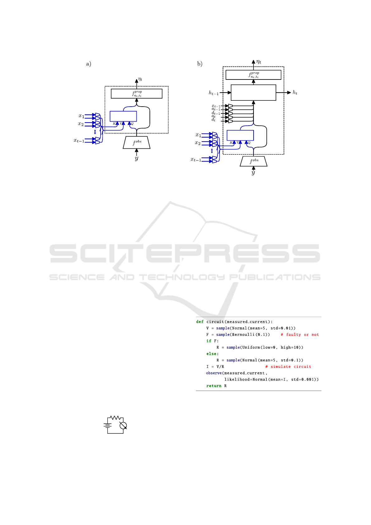
As an example, consider the simple circuit as well

as the probabilistic program shown in Figure 2, which

expresses the joint distribution over the battery volt-

age, V , whether the resistor is faulty, F, the resis-

tance of the resistor, R, and the measured current, I,

as p(V,F,R,I) = p(I|V, R)p(R|F)p(F)p(V ).

Traces will have the form (x

)

T =3

t=1

where

there are two trace “types,” one corresponding to the

sequence of addresses of random variables generated

if the resistor is faulty, and the other the opposite. In

other words a

is the address where V is sampled, a

is the address where F is sampled, and a

is the ad-

dress from which R is sampled, which depends on F.

The instance counts in this program are always i

= i

= 1, and the observation, measured current

∼ N(I,0.001), with N = 1.

This generative model allows posterior inference

to be performed over the joint distribution of the in-

put voltage V , current I, and “faulty” variable F given

the observed measured current. Estimates of the

marginal posterior distribution over F make it possi-

ble to directly answer questions such as whether the

resistor is faulty or not. We will return to a more com-

plex version of this problem in Section 4.3.

Generally, PPLs are designed to infer posterior

distributions over the latent variables given the obser-

vations. Inference in probabilistic programs is car-

ried out with algorithms such as Sequential Impor-

tance Sampling (SIS) (Arulampalam et al., 2002),

Lightweight Metropolis-Hastings (Wingate et al.,

2011), and Sequential Monte Carlo (Del Moral et al.,

2006). However, these algorithms are too computa-

tionally expensive for use in real-time applications.

Therefore, recent research (Le et al., 2017; Kulkarni

et al., 2015) has considered amortizing the computa-

tional cost by performing up-front computation (for a

given model) to allow faster inference later (given this

model and any observed values).

2.2 Inference Compilation

Inference compilation, or IC (Le et al., 2017), is

a method for performing amortized inference in the

framework of universal probabilistic programming.

IC involves training neural networks, which we de-

scribe as “inference networks,” whose outputs pa-

rameterize proposal distributions used for Sequen-

tial Importance Sampling (SIS) (Arulampalam et al.,

2002). IC attempts to match the proposal distribu-

tion, q(x|y; φ) =

∏

t=1

|η

1:t−1

,y,φ)) close to

the true posterior, p(x|y) using the Kullback-Leibler

divergence, D

(p(x|y)||q(x|y;φ)), as a measure of

“closeness”. In order to ensure closeness for any ob-

served y, an expectation of this divergence is taken

with respect to p(y),

L (φ) =E

p(y)

(p(x|y)||q(x|y;φ))]

p(x,y)

[−log q(x|y,φ)] + const. (2)

The parameters, φ, are updated by gradient descent

with the following gradient estimate of (2),

∇

L (φ) ≈

∑

m=1

−∇

logq(x

,φ), (3)

where (x

) ∼ p(x,y) for m = {1,...,M}. Note

that the loss used, and the estimates of the gradi-

ents, are identical to those in the sleep-phase of wake-

sleep (Hinton et al., 1995).

The architecture used in IC (Baydin et al., 2019;

Le et al., 2017) consists of the black components

Attention for Inference Compilation

dot-product

attention

LSTM

...

dot-product

attention

...

Figure 1: Feedforward and LSTM neural network architectures with attention mechanisms. The components inside the dashed

line are run once at each sample statement in a program trace, while the parts outside this line are run only once per trace.

The added attention mechanism is shown in blue.

shown in Figure 1b. Before performing inference,

observations y are embedded by a learned observe

embedder, f

obs

. At each sample statement encoun-

tered as the program runs, the correspondingly LSTM

runs for one time step. It receives an input con-

sisting of the concatenation of the embedding of the

observed values, f

obs

(y), an embedding of x

t−1

, the

value sampled at the previous sample statement, em-

beddings of the current and previous address, instance

and distribution-type. The embedder used for x

t−1

speciﬁc to (a

t−1

), the address and instance from

which x

t−1

was sampled. The output of the LSTM

is fed into a proposal layer, which is speciﬁc to the

address and instance (a

and i

). The proposal layer

outputs the parameters, η

, of a proposal distribution

for the variable at this sample statement.

2.3 Dot-product Attention

Attention has proven useful in a number of tasks, in-

cluding image captioning, machine translation, and

image generation (Xu et al., 2015; Bahdanau et al.,

2014; Gregor et al., 2015). The two broad types of at-

tention are hard and soft attention. Hard attention (Ba

et al., 2014; Xu et al., 2015) selects a single “loca-

tion” to attend to, and thus requires only this location

to be embedded. However, it is non-differentiable. In

contrast, soft attention mechanisms (Vaswani et al.,

Figure 2: The electronic circuit modelled by the probabilis-

tic program in Figure 3.

2017; Xu et al., 2015) are fully differentiable and here

we focus especially on dot-product attention (Luong

et al., 2015; Vaswani et al., 2017).

The dot-product attention module (Luong et al.,

2015; Vaswani et al., 2017), shown in Figure 5, re-

ceives three inputs: one or more query vectors (which

describe the desired properties of the locations to at-

tend to), a key vector for each location, and a value

vector for each location; these are represented as the

matrices Q ∈ R

q×k

, K ∈ R

k×l

, and V ∈ R

l×v

respec-

tively. Note that in our context a location corresponds

to a previously sampled value. Here, l is the number

of locations, k is the length of each query and key em-

bedding, v is the length of each value embedding, and

q is the number of queries. For each query, attention

Figure 3: Probabilistic program modeling the circuit in Fig-

ure 2 with a possibly faulty resistor. First the voltage, V ,

of the battery is sampled from a Gaussian prior centered on

5V. We then sample whether or not the resistor is faulty. If

it is, its value is sampled from a broad uniform distribution.

Otherwise, its value is sampled from a tightly peaked Gaus-

sian. A noisy measurement of the current is then sampled

from a Gaussian prior centered on the true value.

SIMULTECH 2022 - 12th International Conference on Simulation and Modeling Methodologies, Technologies and Applications

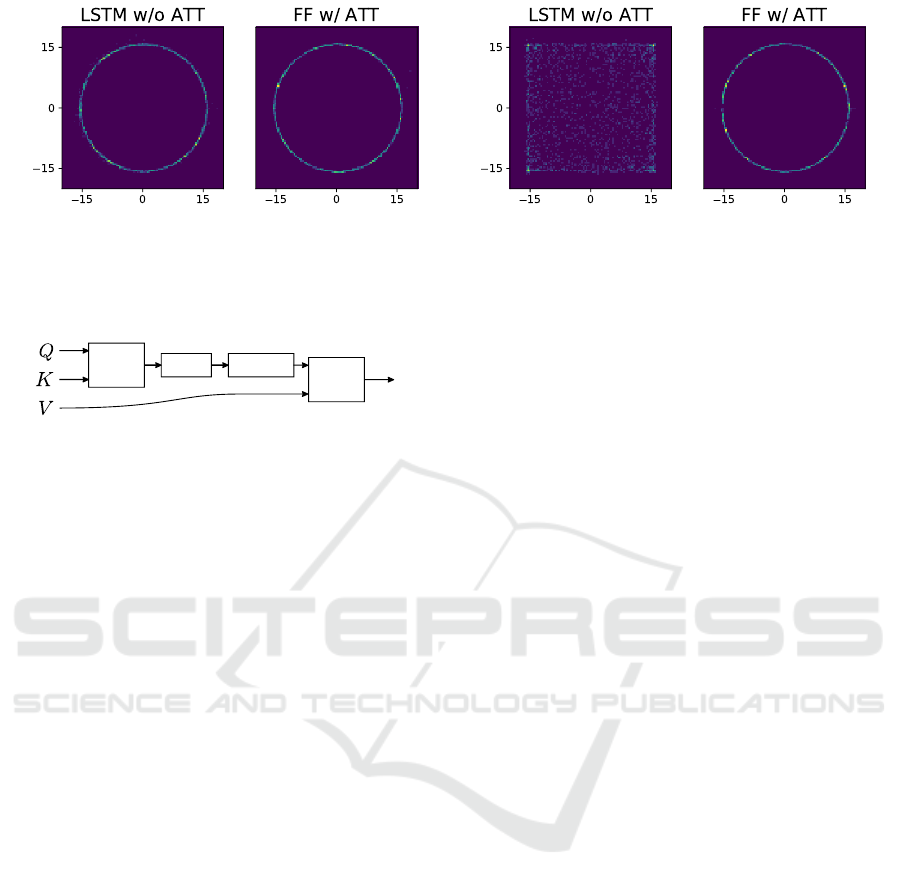
(a) Model with 20 nuisance variables. (b) Model with 50 nuisance variables.

Figure 4: 2000 samples from the proposal distributions of each of an LSTM-based inference network and an attention-based

network. The LSTM is able to learn the dependence of y on x when they are separated by 20 nuisance variables, but fails

when this is increased to 50. The attention mechanism can handle either case.

SoftMax

MatMul

Scale

Figure 5: A scaled dot-product attention mechanism. Figure

adapted from (Vaswani et al., 2017).

weights are computed for every location by taking the

dot-product of the query vector and the relevant key.

3 METHOD

We augment both the LSTM and feedforward archi-

tectures with dot-product attention over all previously

sampled variables, as shown in Figure 1. Although

soft attention is, in many cases, vastly more computa-

tionally expensive than hard attention, this is not the

case for our application; since the embedding of each

sampled value can be used at every later time step, the

cost of calculating these embeddings scales only lin-

early with trace length. This is no worse than the rate

that hard attention achieves. We therefore use soft at-

tention for the ease of training.

During training we build a data structure, d

k,v,q

with associative mappings linking address/instance

pairs (a,i) to key, value and query embedders. The

embedders in d

k,v,q

are constructed dynamically for

each new address and instance pair (a

) encoun-

tered. During inference, the queries, keys, and values

fed to the attention mechanism at each sample state-

ment are calculated as follows: for the ﬁrst sample

statement, identiﬁed by (a

), no previously sam-

pled variables exist and so the attention module out-

puts a vector of zeros. Using the associated key and

value embedders in d

k,v,q

, the variable sampled, x

is embedded to yield a key and a value, k

and v

) are kept in memory throughout the trace, al-

lowing fast access for subsequent sample statements.

The second sample statement can attend to the ﬁrst

sampled variable via (k

) using a query. The em-

bedder used for ﬁnding the query takes as input the

observe embedding, f

obs

(y), and is speciﬁc to the

current address and instance (a

). As with the

key/value embedders, the query embedder is found in

k,v,q

. The output of the attention module is then fed

to the LSTM or proposal layer (see Figure 1). As for

, x

is sampled and embedded using the embedders

stored in d

k,v,q

, yielding the key, value pair (k

This procedure is repeated until the end of the trace,

as deﬁned by the probabilistic program. In the con-

text of higher-order programs, an address and instance

pair may be encountered during inference that has not

been seen during training. In this case the proposal

layers have not been trained, and so the standard IC

approach is to use the prior as a proposal distribution.

For the same reason, the key/value embedders do not

exist and so no keys or values are created for this

). This prevents later sample statements from

attending to the variable sampled at (a

4 EXPERIMENTS

We consider feedforward and LSTM architectures

both with and without attention, which we de-

note FF w/o ATT, FF w/ ATT, LSTM w/o ATT and

LSTM w/ ATT. We compare them through experi-

ments with inference in three probabilistic programs:

a pedagogical example to illustrate a failure case of

the LSTM architecture; a model of gene expression

in plants; and ﬁnally an electronic circuit simulator.

We implement our proposed architecture in, and per-

form the experiments using, pyprob (Le et al., 2017;

Baydin and Le, 2018), a probabilistic programming

language designed for IC. All experiments use the

same attention mechanism hyperparameters: q = 4,

k = 16 and v = 8. We also use pyprob’s default neu-

ral network layer sizes, optimizer (Adam (Kingma

and Ba, 2014)) and associated hyperparameters, batch

Attention for Inference Compilation

Figure 6: Fifth-order band-pass Butterworth ﬁlter with resistors, capacitors and inductors denoted by R, C, and L respectively.

The dashed lines represent possible short circuits. The existence of these short circuits and whether or not each component

is faulty (represented by a noisy component value) or disconnected is sampled according to the generative model. Given

observations of V

out

for various input frequencies, the task is to infer a distribution over possible faults such as short circuits

and poorly connected or incorrectly valued components.

0.00

0.05

0.10

0.15

AC Voltage (V)

ESS =1.2±0.27

FF w/o ATT

ESS =1.9±0.47

LSTM w/o ATT

ESS =3.3±1.19

FF w/ ATT

Proposal

ESS =2.3±0.73

LSTM w/ ATT

980 1000 1020

f (Hz)

0.00

0.02

0.04

0.06

AC Voltage (V)

980 1000 1020

f (Hz)

980 1000 1020

f (Hz)

980 1000 1020

f (Hz)

Estimated Posterior

Observations Samples

Figure 7: Reconstruction of the output voltage using samples from each proposal distribution. In the architectures with

attention, the sampled voltages are almost all close to the observations (green ‘x’s) whereas, without attention, the proposals

place high probability in regions which do not ﬁt the observations. These better proposal distributions lead the higher effective

sample sizes shown in each ﬁgure (mean and standard deviation, calculated with 5 estimates). The proposal distribution is

shown using 100 samples from each architecture.

FF w/o ATT LSTM w/o ATT FF w/ ATT LSTM w/ ATT Ground truth

None

C4 short

C2 short

Multiple

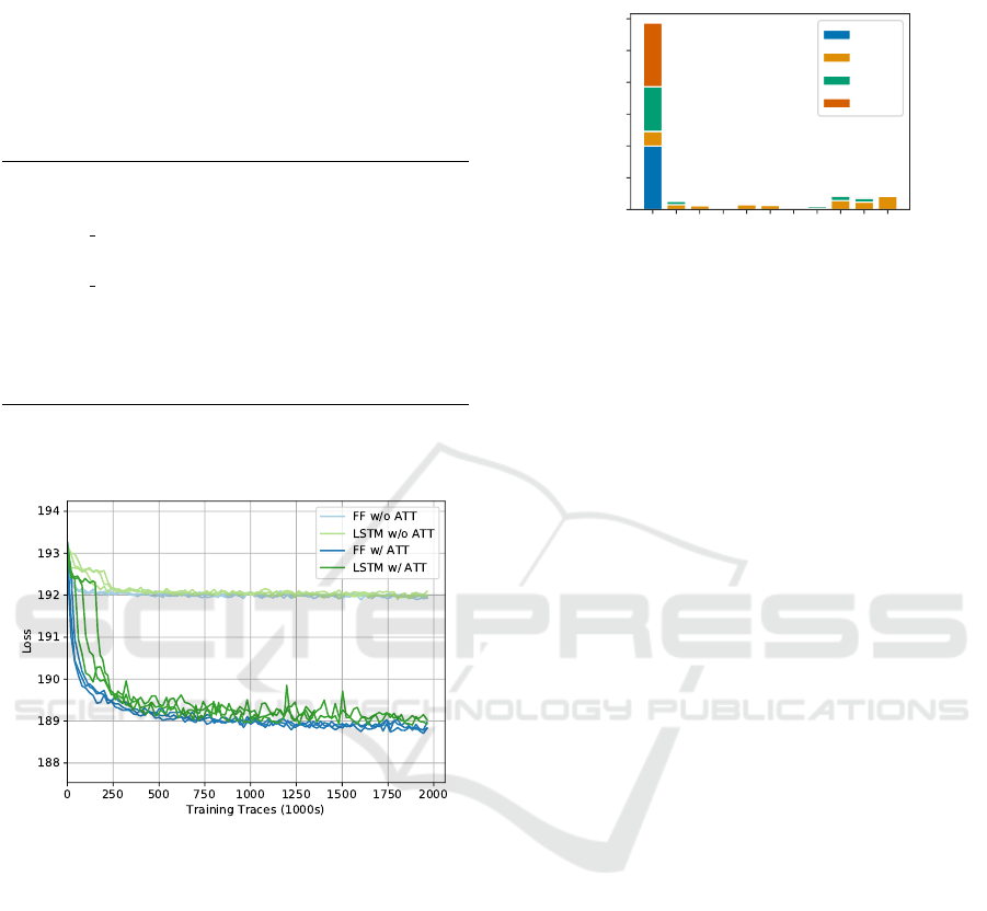
Figure 8: A visualisation of the proposal distributions given some observation sampled from the model. The pie charts show

the probability of different possibilities: that there are no faults, multiple faults, or one of multiple speciﬁc types of fault. For

each architecture, 1000 unweighted samples are shown. A ‘ground truth’ posterior, created with 10 000 importance-weighted

sampled from LSTM w/o ATT, is shown to the right. Since it is probable that exactly one of the faults ‘C2 short’ or ‘C4 short’

has occured, there is a dependence between these two variables. Either an LSTM or an attention mechanism (or both) can be

seen to be sufﬁcient to capture this dependence (thus reducing the error of the weighted posterior approximation). The error

is calculated by embedding the samples as a vector where each element corresponds to a possible fault and is 1 if this fault is

present, or 0 otherwise. The L2-Wasserstein distance from the ground truth is then measured.

size (64) and learning rate (10

−3

). The only exception

to this is that a learning rate of 10

−4

was used to sta-

bilise training of the gene expression model.

4.1 Magnitude of Random Vector

Our ﬁrst program samples two latent variables, x

and y, from identical and independent normal dis-

tributions, N(0,σ

). An observation of x

+ y

then made with Gaussian noise, and denoted ˆr

∼

N(ˆr

+ y

,σ

). We wish to infer the posterior over

x and y conditioned on this. We use σ

= 10 and

= 0.5, giving a peaked posterior exhibiting circular

symmetry, and so a strong dependence between x and

y. To test the inference network’s ability to capture

long-term dependencies, we sample “nuisance” vari-

ables between sampling x and y. These are not used

elsewhere in the program, serving only to increase the

“distance” between x and y. We provide pseudocode

for this program in the appendix.

All inference networks for this model are trained

for 2000 000 traces. Figure 4 shows samples of x

and y from learned proposal distributions for two pro-

grams with different numbers of nuisance variables

(which are marginalized out). The inference network

with an attention mechanism can be seen to learn the

dependency even with 50 nuisance variables, while

the LSTM cannot.

SIMULTECH 2022 - 12th International Conference on Simulation and Modeling Methodologies, Technologies and Applications

4.2 Plant Gene Expression

We consider a model of gene expression for Ara-

bidopsis thaliana, a small plant. This was presented

by (Opgen-Rhein and Strimmer, 2007) as a Bayesian

network, and we write it as a probabilistic program.

Although this model has simple link functions (each

node is normally distributed with mean given by an

afﬁne function of the values of parent nodes), it tests

the ability of each architecture to learn a dependency

structure from a real-world simulator. The network

contains 107 nodes and 150 edges. We randomly se-

lect 40 of the 67 leaf nodes to be observable, and at-

tempt to infer the values of all other nodes given these.

We train inference networks for 4 000 000 traces for

this model. Visualizations of the attention weights for

this model and the magnitude model are in the ap-

pendix.

4.3 Electronic Circuit Fault Diagnosis

The ﬁnal probabilistic program we consider is a

model of an electronic circuit (speciﬁcally, a band-

pass Butterworth ﬁlter). The model samples many

random variables describing the components values

and the existence of possible faults (such as short-

circuits or missing components). A pre-existing cir-

cuit simuator (Venturini et al., 2017) then generates

the complex-valued output voltage (i.e. voltage mag-

nitude and phase) at 40 different input frequencies.

Given an observation of this (under Gaussian noise),

we infer what faults, if any, exist. An illustration of

the Butterworth ﬁlter can be found in Fig. 6. The in-

ference networks are trained for 3000 000 traces.

To perform inference we write a probabilistic pro-

gram (see appendix) that iterates through each com-

ponent of the circuit and samples in the following or-

der: ﬁrst, whether or not it is correctly connected to

the rest of the circuit. Second, the component value

is sampled from a mixture of a broad uniform distri-

bution and a tightly peaked Gaussian, both centered

on the nominal value. The value is sampled from

the tightly peaked Gaussian with 98% probability and

from the uniform distribution with 2% probability.

Conceptually, one can interpret the tightly peaked

Gaussian as the distribution given that the component

has been correctly made. The broad uniform distri-

bution represents the distribution for components that

are faulty.

To test each inference network, we generate 100

different observations by running the probabilistic

program, and attempt to infer the posterior using

each different network architecture. For each in-

ference network architecture, we estimate the pos-

terior distribution 5 times using importance sam-

pling with 20 traces each time. Across the 5 es-

timates, we compute the average ESS, and average

these over all 100 observations. The averaged results

were 1.40 for FF w/o ATT, 7.26 for LSTM w/o ATT,

8.46 for FF w/ ATT and 8.35 for LSTM w/ ATT. The

attention-based architecture has an 16.5% higher av-

erage ESS than the LSTM core, showing that the use

of attention leads to quantitatively better proposal dis-

tributions.

We further ﬁnd that whenever the observed signal

appears to originate from a correctly working Butter-

worth ﬁlter, all architectures seem to produce reason-

able predictive posterior distributions - i.e. the dis-

tribution of the voltage signal generated by the sam-

pled latent variables. However, the attention-based

architectures yield a higher average ESS with only

a few exceptions. When the observed signal clearly

originates from an erroneous ﬁlter, M

FF w/o ATT

pro-

duces predictive posterior distributions which poorly

ﬁt the observed data. The LSTM-based architecture

produces better predictive posterior distributions but

these are still signiﬁcantly worse than the distribu-

tions produced by the attention-based architecture in

almost all cases where the ﬁlter is broken.

Figure 7 shows inference performance for one

such observation originating from a ﬁlter in which

the component is faulty. We plot voltages gener-

ated according to the sampled latent variables from

the predictive proposal distributions using each ar-

chitecture. The proposals from FF w/ ATT and

LSTM w/ ATT are clustered near to the observations,

whereas FF w/o ATT and LSTM w/o ATT produce

many proposals that do not ﬁt the observations.

We suspect that these outliers occur due to the in-

ability of M

FF w/o ATT

and M

LSTM w/o ATT

to learn long-

range dependencies. For example, an output volt-

age of zero could be explained by a number of dif-

ferent faults (e.g. a short-circuit across C

or across

). If the resulting dependency between these can be

learned, the proposals could consistently predict that

only one is broken (predicting more would be unlikely

due to the strong prior on parts working). However, if

the dependency is not captured, the proposals would

be prone to predicting that zero or multiple compo-

nents are broken. This interpretation is supported by

Figure 7, where both architectures without attention

are seen to sometimes propose an output voltage cor-

responding closely to a working circuit.

Figure 8 shows an example of the posterior dis-

tributions inferred over possible faults by each archi-

tecture. For this purpose, a component is considered

faulty when its value is outside of a 0.3% tolerance

of its nominal value. The architectures with attention

Attention for Inference Compilation

(a) Magnitude (20 nuisance var.).

(b) Plant gene expression model.

Figure 9: Loss, E

p(x,y)

[−log q(x|y,φ)], throughout training for each model and architecture. To reduce noise, the losses are

averages over batches of 468 training steps. Runs with 3 different random seeds are shown. Due to space constraints, the plot

for the magnitude model with 50 nuisance variables is in the appendix.

Table 1: Milliseconds per inference trace for each model and architecture, using a node with 8 CPU cores. Measurements are

averaged over 10 runs of inference, with each drawing 100 samples.

FF w/o ATT LSTM w/o ATT FF w/ ATT LSTM w/ ATT

Magnitude of r.v. 20 74.1 86.5 89.6 104

Magnitude of r.v. 50 161 200 198 236

Plant gene expression 233 282 282 324

Electronic circuit faults 121 140 145 173

manage to most closely ﬁt the ground truth posterior.

4.4 Analysis

Fig. 9 shows the loss of each network throughout

training. In every case, the feedforward network with

attention performs at least as well as the LSTM-based

architecture without attention. In particular, the at-

tention model achieves a signiﬁcantly better ﬁnal loss

for the plane gene expression model. The plot for

the magnitude model with 50 nuisance variables, in

which attention also gives an improved ﬁnal loss, is

in the appendix. When only 20 nuisance variables are

used, the architecture with attention trains faster but

to a similar ﬁnal loss. We also observe that, in our ex-

periments, using an LSTM and attention in conjunc-

tion never provides a signiﬁcant improvement over

using attention alone, while being more computation-

ally costly.

Table 1 shows the time taken to run each archi-

tecture. Magnitudes 20 and 50 have 22 and 52 la-

tent variables respectively, the plant gene simulator

has 67, and the circuit simulator typically encounters

43. Since each variable is proposed sequentially, in-

ference takes time proportional to the number of la-

tent variables. The computational cost of the attention

mechanism is similar to that of the LSTM. Also, al-

though the cost of calculating attention weights, and

thus the runtime of the attention mechanism, theoreti-

cally scales as the square of the trace length while the

LSTM’s runtime scales linearly, their runtimes scale

similarly in these experiments.

5 DISCUSSION AND

CONCLUSION

We have demonstrated that the standard LSTM core

used in IC can fail to capture long-range dependen-

cies between latent variables. To address this, we

have proposed an attention mechanism which attends

to the most salient previously sampled variables in an

execution trace. We show that this architecture can

speed-up training and sometimes improve the quality

of the learned proposal distributions (measured by the

KL divergence loss), while we never observe it harm-

ing them. These advantages come at negligible com-

putational cost. We believe this makes the attention-

based architecture a sensible default choice for new

inference problems. Future work could consider ex-

tending the usage of such an attention mechanism to

also attend to observed variables. The inference com-

pilation framework is only applicable to models with

a ﬁxed number of observations, but such an attention

mechanism may allow this requirement to be relaxed.

REFERENCES

Arulampalam, M., Maskell, S., Gordon, N., and Clapp,

T. (2002). A tutorial on particle ﬁlters for online

SIMULTECH 2022 - 12th International Conference on Simulation and Modeling Methodologies, Technologies and Applications

nonlinear/non-gaussian bayesian tracking. Ieee Trans-

actions on Signal Processing, 50(2):174–188.

Ba, J., Mnih, V., and Kavukcuoglu, K. (2014). Multiple ob-

ject recognition with visual attention. arXiv preprint

arXiv:1412.7755.

Bahdanau, D., Cho, K., and Bengio, Y. (2014). Neural ma-

chine translation by jointly learning to align and trans-

late. arXiv preprint arXiv:1409.0473.

Baydin, A. G. and Le, T. A. (2018). pyprob.

Baydin, A. G., Shao, L., Bhimji, W., Heinrich, L., Naderi-

parizi, S., Munk, A., Liu, J., Gram-Hansen, B.,

Louppe, G., Meadows, L., et al. (2019). Efﬁcient

probabilistic inference in the quest for physics beyond

the standard model. In Advances in Neural Informa-

tion Processing Systems, pages 5460–5473.

Bingham, E., Chen, J. P., Jankowiak, M., Obermeyer, F.,

Pradhan, N., Karaletsos, T., Singh, R., Szerlip, P.,

Horsfall, P., and Goodman, N. D. (2018). Pyro: Deep

Universal Probabilistic Programming. arXiv preprint

arXiv:1810.09538.

Del Moral, P., Doucet, A., and Jasra, A. (2006). Sequen-

tial monte carlo samplers. Journal of the Royal Sta-

tistical Society: Series B (Statistical Methodology),

68(3):411–436.

Gershman, S. and Goodman, N. (2014). Amortized infer-

ence in probabilistic reasoning. In Proceedings of the

Annual Meeting of the Cognitive Science Society, vol-

ume 36.

Goodman, N. D., Mansinghka, V. K., Roy, D., Bonawitz,

K., and Tenenbaum, J. B. (2008). Church: A language

for generative models. Proceedings of the 24th Con-

ference on Uncertainty in Artiﬁcial Intelligence, Uai

2008, pages 220–229.

Gregor, K., Danihelka, I., Graves, A., Rezende, D. J.,

and Wierstra, D. (2015). Draw: A recurrent neu-

ral network for image generation. arXiv preprint

arXiv:1502.04623.

Hinton, G. E., Dayan, P., Frey, B. J., and Neal, R. M. (1995).

The” wake-sleep” algorithm for unsupervised neural

networks. Science, 268(5214):1158–1161.

Hochreiter, S. and Schmidhuber, J. (1997). Long short-term

memory. Neural Computation, 9(8):1735–1780.

Jaderberg, M., Simonyan, K., Zisserman, A., et al. (2015).

Spatial transformer networks. In Advances in neural

information processing systems, pages 2017–2025.

Kingma, D. P. and Ba, J. (2014). Adam: A

method for stochastic optimization. arXiv preprint

arXiv:1412.6980.

Kulkarni, T. D., Kohli, P., Tenenbaum, J. B., and Mans-

inghka, V. (2015). Picture: A probabilistic program-

ming language for scene perception. In Proceedings

of the ieee conference on computer vision and pattern

recognition, pages 4390–4399.

Le, T. A., Baydin, A. G., and Wood, F. (2017). Inference

compilation and universal probabilistic programming.

In Proceedings of the 20th International Conference

on Artiﬁcial Intelligence and Statistics, volume 54

of Proceedings of Machine Learning Research, pages

1338–1348, Fort Lauderdale, FL, USA. PMLR.

Luong, M.-T., Pham, H., and Manning, C. D. (2015). Ef-

fective approaches to attention-based neural machine

translation. arXiv preprint arXiv:1508.04025.

Mansinghka, V., Selsam, D., and Perov, Y. (2014). Ven-

ture: a higher-order probabilistic programming plat-

form with programmable inference. arXiv preprint

arXiv:1404.0099.

Milch, B., Marthi, B., Russell, S., Sontag, D., Ong, D. L.,

and Kolobov, A. (2005). Blog: Probabilistic models

with unknown objects. Ijcai International Joint Con-

ference on Artiﬁcial Intelligence, pages 1352–1359.

Minka, T., Winn, J., Guiver, J., Zaykov, Y., Fabian, D., and

Bronskill, J. (2018). /Infer.NET 0.3. Microsoft Re-

search Cambridge. http://dotnet.github.io/infer.

Munk, A.,

Scibior, A., Baydin, A. G., Stewart, A., Fern-

lund, G., Poursartip, A., and Wood, F. (2019). Deep

probabilistic surrogate networks for universal simula-

tor approximation. arXiv preprint arXiv:1910.11950.

Opgen-Rhein, R. and Strimmer, K. (2007). From cor-

relation to causation networks: a simple approxi-

mate learning algorithm and its application to high-

dimensional plant gene expression data. BMC systems

biology, 1(1):37.

Seo, M., Kembhavi, A., Farhadi, A., and Hajishirzi, H.

(2016). Bidirectional attention ﬂow for machine com-

prehension. arXiv preprint arXiv:1611.01603.

Tran, D., Kucukelbir, A., Dieng, A. B., Rudolph, M., Liang,

D., and Blei, D. M. (2016). Edward: A library for

probabilistic modeling, inference, and criticism. arXiv

preprint arXiv:1610.09787.

van de Meent, J.-W., Paige, B., Yang, H., and Wood, F.

(2018). An introduction to probabilistic programming.

arXiv preprint arXiv:1809.10756.

Vaswani, A., Shazeer, N., Parmar, N., Uszkoreit, J., Jones,

L., Gomez, A. N., Kaiser, Ł., and Polosukhin, I.

(2017). Attention is all you need. In Advances in

Neural Information Processing Systems, pages 5998–

6008.

Venturini, G., Daniher, I., Crowther, R., and KOLANICH

(2017). ahkab.

Wingate, D., Andreas Stuhlm

uller, A., and Goodman, N. D.

(2011). Lightweight implementations of probabilis-

tic programming languages via transformational com-

pilation. Journal of Machine Learning Research,

15:770–778.

Wood, F., Meent, J. W., and Mansinghka, V. (2014). A

new approach to probabilistic programming inference.

In Artiﬁcial Intelligence and Statistics, pages 1024–

1032.

Xu, K., Ba, J., Kiros, R., Cho, K., Courville, A., Salakhudi-

nov, R., Zemel, R., and Bengio, Y. (2015). Show, at-

tend and tell: Neural image caption generation with

visual attention. In International Conference on Ma-

chine Learning, pages 2048–2057.

Attention for Inference Compilation

APPENDIX

Magnitude of Random Vector

Psuedocode

Program 1: Generative model for the magnitude of a ran-

dom vector with M nuisance random variables.

def magnitude (obs, M):

x = sample(Normal (0, 10))

for in range(M):

# nuisance variables to extend trace

= sample(Normal (0,10))

y = sample(Normal (0,10))

observe(obs

Likelihood = Normal(x

+ y

, 0.1))

return x, y

Additional Training Plot

Figure 10: Loss curve for various inference networks for the

“Magnitude of random variable” model with 50 nuisance

variables.

Attention Weights

Variable Attended to When Sampling y

0.0

0.5

1.0

1.5

2.0

2.5

3.0

Weight

E(w

)

E(w

)

E(w

)

E(w

)

Figure 11: Attention weights used on each previously sam-

pled variable when creating a proposal distribution for y in a

version of the magnitude model with 10 nuisance variables.

Each color represents one of the four queries. The weights

are averaged over 100 traces. Queries 1 and 4 attend solely

to x, explaining how the attention mechanism enables the

inference network to capture the long-term dependency, and

ignore the nuisance variables.

SIMULTECH 2022 - 12th International Conference on Simulation and Modeling Methodologies, Technologies and Applications

Plant Gene Expression Model

Attention Weights

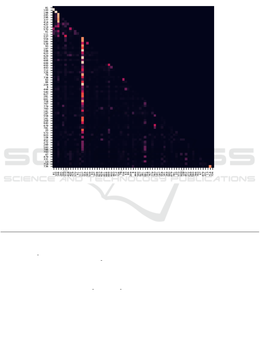
Figure 12: Attention weights used by an FF w/ ATT inference network on the plant gene expression model. The cells in each

row i correspond to the weight given to previously sampled variable when variable i is being sampled. The node numbers

correspond to (Opgen-Rhein and Strimmer, 2007).

Electronic Circuit Fault Diagnosis

Program 2: Generative model for the Butterworth ﬁlter.

class Butterworth ( Model ):

@staticmethod

def sample componen t ( name , mean ,

std =None , p broken =0.02):

if std is None:

std = 0.001

mean

broken = pyprob.sample(

dist.Categorical (

torch.tensor ([1−p broken , p broke n ])

)). item()

if broken:

r = pyprob.sample(

dist.Uniform ( torch . tensor ([0.]) ,

torch.tensor ([2.]))). item()

val = r

torch.tensor ([ mean])

else:

r = pyprob.sample(

Attention for Inference Compilation

dist.Normal(torch.tensor (0) ,

torch.tensor (1))). item()

val = mean + r

std

return max(val , 1e −16)

@staticmethod

def sample erro r ( name , p =0.005):

return bool(

pyprob.sample(

dist.Categorical (

torch.tensor ([1−p , p]))). item ())

def forward ( self):

cir = Circuit (’Butterworth 1kHz band −pass filter ’)

R1 = self.sample componen t (’R1’, mean=50.)

R1 open = self.sample error(’R1open ’)

L1 = self.sample componen t (’L1’, mean =0.245894)

L1 open = self.sample error(’L1open ’)

C1 = self.sample componen t (’C1’, mean=1.03013 e−07)

L2 = self.sample componen t (’L2’, mean=9.83652 e−05)

L2 open = self.sample error(’L2open ’)

C2 = self.sample componen t (’C2’, mean =0.000257513)

C1 open = self.sample error(’C1open ’)

if self .sample e rro r ( ’C1short ’):

cir . add resis tor (’Rshort2 ’, ’n3 ’, ’n4’, 0.001)

C2 open = self.sample error(’C2open ’)

if self .sample e rro r ( ’C2short ’):

cir . add resis tor (’Rshort2 ’, ’n4 ’, cir .gnd , 0.001)

C3 open = self.sample error(’C3open ’)

C4 open = self.sample error(’C4open ’)

L3 = self.sample componen t (’L3’, mean =0.795775)

L3 open = self.sample error(’L3open ’)

C3 = self.sample componen t (’C3’, mean=3.1831e−08)

Vin broke n = self.sample erro r ( ’ Vin broken ’)

if self .sample e rro r ( ’C3short ’):

cir . add resis tor (’Rshort3 ’, ’n5 ’, ’n6’, 0.001)

C5 open = self.sample error(’C5open ’)

L4 = self.sample componen t (’L4’, mean=9.83652 e−05)

L4 open = self.sample error(’L4open ’)

C4 = self.sample componen t (’C4’, mean =0.000257513)

if self .sample e rro r ( ’C4 ’):

cir . add resis tor (’Rshort4 ’, ’n6 ’, cir .gnd , 0.001)

C5 = self.sample componen t (’C5’, mean=1.03013 e−07)

C5 open = self.sample error(’C5open ’)

if self .sample e rro r ( ’C5 ’):

cir . add resis tor (’Rshort5 ’, ’n7 ’, ’n8’, 0.001)

L5 open = self.sample error(’L5open ’)

R2 open = self.sample error(’R2open ’)

L5 = self.sample componen t (’L5’, mean =0.245894)

R2 = self.sample componen t (’R2’, mean=50.)

if not Vin bro ken :

cir . add vsource (’V1 ’, ’n1 ’, cir.gnd , dc v alu e =0. , ac va lue =1.)

if not R1 op en :

cir . add resis tor (’R1 ’, ’n1 ’, ’n2’, R1)

if not L1 op en :

cir . add induc tor (’L1 ’, ’n2 ’, ’n3’, L1)

if not C1 op en :

cir . add capacitor(’C1 ’, ’n3 ’, ’n4’, C1)

if not L2 op en :

cir . add induc tor (’L2 ’, ’n4 ’, cir.gnd , L2)

if not C2 op en :

cir . add capacitor(’C2 ’, ’n4 ’, cir.gnd , C2)

SIMULTECH 2022 - 12th International Conference on Simulation and Modeling Methodologies, Technologies and Applications

if not L3 op en :

cir . add induc tor (’L3 ’, ’n4 ’, ’n5’, L3)

if not C3 op en :

cir . add capacitor(’C3 ’, ’n5 ’, ’n6’, C3)

if not L4 op en :

cir . add induc tor (’L4 ’, ’n6 ’, cir.gnd , L4)

if not C4 op en :

cir . add capacitor(’C4 ’, ’n6 ’, cir.gnd , C4)

if not C5 op en :

cir . add capacitor(’C5 ’, ’n7 ’, ’n8’, C5)

if not L5 op en :

cir . add induc tor (’L5 ’, ’n6 ’, ’n7’, L5)

if not R2 op en :

cir . add resis tor (’R2 ’, ’n8 ’, cir.gnd , R2)

else:

cir . add resis tor (’R2 ’, ’n8 ’, cir.gnd , R2

1000)

# analysis

ac1 = new ac (.97e3 , 1.03e3 , 40 , x0 =None)

res = run (cir , ac 1 )[’ac’]

vouts = res [’Vn8’]

rs = abs( vouts )

thetas = np.angle(vouts)

# observations

pyprob.observe( dist.Normal ( torch . tensor(rs ), torch. tensor (0.03)),

name=’ | Vout | ’)

pyprob.observe( dist.Normal ( torch . tensor(thetas), torch . tensor(0.05)) ,

name=’ theta o ut ’)

Attention for Inference Compilation