Bridging the Gap between Real and Synthetic Trafﬁc Sign Repositories

Diogo Lopes da Silva

and Ant

onio Ramires Fernandes

2 a

Universidade do Minho, Braga, Portugal

Algoritmi Centre/Department of Informatics, Universidade do Minho, Braga, Portugal

Keywords:

Synthetic Training Sets, Trafﬁc Sign Classiﬁcation Repositories, Convolutional Neural Networks.

Abstract:

Current trafﬁc sign image repositories for classiﬁcation purposes suffer from scarcity of samples due to the

compiling and labelling images being mainly a manual process. Thus, researchers resort to alternative ap-

proaches to deal with this issue, such as increasing the model architectural complexity or performing data

augmentation. A third approach is the usage of synthetic data. This work addresses the data shortage issue by

building a synthetic repository proposing a pipeline to build synthetic samples introducing previously unused

image operators. Three use cases for synthetic data usage are explored: as a standalone training set, merging

with real data, and ensembling. The ﬁrst option provides results that not only clearly surpass any previous

attempt on using synthetic data for trafﬁc sign recognition but are also encouragingly placing the obtained ac-

curacies closer to results with real images. Merging real and synthetic data in a single data set further improves

those results. Due to the different nature of the datasets involved, ensembling provides a boost in accuracy

results. Overall we got results in three different datasets that surpass previous state of the art results: GTSRB

(99.85%), BTSC (99.76%), and rMASTIF (99.84%). Finally, cross testing amongst the three datasets hints

that our synthetic datasets have the potential to provide better generalization ability than using real data.

1 INTRODUCTION

Typically, training deep learning models requires a

high volume of samples. In the context of trafﬁc sign

recognition, collecting a truly representative dataset

is both a time and resource consuming task. For in-

stance, some trafﬁc signs appear only in highways

while others appear only in rural areas. Furthermore,

these signs should be captured in a wide range of

lighting and weather conditions, as well as using dif-

ferent camera sensors. When all factors are taken into

account, the process of building a truly representative

dataset of real-world images is not to be taken lightly.

To aggravate things further, it must be taken into

account that a model trained with trafﬁc signs from

a speciﬁc country will not be optimal when used in

a different country. Small differences in letter fonts

and pictograms are sufﬁcient to signiﬁcantly decrease

the accuracy of a model. This issue can also be found

within each country, where pictograms used in traf-

ﬁc signs are sometimes updated or have their font

changed.

Some works address the accuracy problem from

the model architecture perspective. Complex ar-

https://orcid.org/0000-0002-3680-572X

chitectures, namely Spatial Transformer Networks

(STN), Inception modules, and Generative Adversar-

ial Networks (GAN), have been able to achieve con-

siderable accuracies.

The purpose of this work is to address the issues

pertaining to the datasets. We explore the construc-

tion of a dataset based only on synthetic data, thereby

eliminating the data gathering and labelling issues, re-

moving the limitation on the number of classes, and

issues with multiple variations of the same sign.

The only input we require to build a synthetic

dataset is a set of templates that represent the trafﬁc

sign classes to be included. Most of these can be col-

lected from a number of sources on the internet. Note

that for a particular class there may be more than one

template to accommodate older versions of a sign, or

slight variations found by different sign makers.

If real-world data is available, synthetic data can

be used to complement the training set, providing a

hard to obtain diversity when considering only real

samples, thereby potentially increasing the overall

classiﬁcation accuracy.

To evaluate the potential of such datasets, tests

were performed against state-of-the-art reports on

three European trafﬁc sign repositories, considering

Lopes da Silva, D. and Fernandes, A.

Bridging the Gap between Real and Synthetic Trafﬁc Sign Repositories.

DOI: 10.5220/0011301100003277

In Proceedings of the 3rd International Conference on Deep Learning Theory and Applications (DeLTA 2022), pages 44-54

ISBN: 978-989-758-584-5; ISSN: 2184-9277

Table 1: Statistics for the German, Belgian, and Croatian

datasets.

GTSRB BTSC rMASTIF

class # 43 62 31

train # 39209 4575 4044

test # 12630 2520 1784

min res 25x25 22x21 17x16

max res 232x266 674x527 185x159

three usage scenarios: the synthetic dataset as a stan-

dalone training set, merged with a real training set,

and having synthetic and real data participating in

an ensemble. To assess the generalisation ability

of the trained models with synthetic data, we also

performed cross-testing with synthetic data amongst

three datasets.

2 RELATED WORK

This section focuses on the European trafﬁc sign

repositories used in this work, the research litera-

ture using deep learning models trained with these

datasets, and on research relating to synthetic trafﬁc

sign datasets.

2.1 Trafﬁc Sign Datasets

Only for a few countries have trafﬁc sign samples

been collected, labelled, and released as a public

dataset. The volume and quality of samples varies

greatly across countries.

Here we focus on three European datasets: GT-

SRB

(Stallkamp et al., 2012); BTSC

dataset (Timo-

fte et al., 2009); and rMASTIF

dataset (

Segvic et al.,

2010).

Table 1 presents some statistics for these datasets.

2.2 Trafﬁc Sign Classiﬁcation

In 2011, Cires¸an et al. (Cires¸an et al., 2012) won

the IJCNN competition with an ensemble of 25

CNNs. The dataset was preprocessed using 4 differ-

ent colour/brightness equalisation settings, providing

a total of 5 different datasets (including the original).

Each dataset version was used to train 5 models, re-

sulting in 25 trained CNNs. They achieved an accu-

racy of 99.46% in the GTSRB dataset.

In 2015, Haloi (Haloi, 2015) achieved an accuracy

of 99.81% on the GTSRB dataset using a CNN con-

sisting in sequential STN layers along with a modiﬁed

http://benchmark.ini.rub.de/

https://btsd.ethz.ch/shareddata/

http://www.zemris.fer.hr/ kalfa/Datasets/rMASTIF/

version of GoogLeNet, based on an Inception archi-

tecture (Szegedy et al., 2014).

Juri

c et al. (Juri

c et al., 2015) reports an ac-

curacy of 98.17 ± 0.22% on the BTSC dataset and

99.53± 0.10% on the MASTIFF dataset. Their model

was based on the one used by Cires¸an et al.(Cires¸an

et al., 2012), and included width branches (also

named scales) of convolutional layers in order to cre-

ate a multi-scale architecture in a similar approach to

the work of (Sermanet and LeCun, 2011).

Later, Arcos-Garc

ıa et al. (Arcos-Garc

ıa et al.,

2018) accomplished a performance of 99.71% on the

GTSRB dataset and 98.95% on the BTSC dataset.

Their architecture consists in a single CNN that com-

bines convolutional layers and 3 STN modules.

In 2018, the performance on the BTSC was im-

proved by Saha et al. (Saha et al., 2018) achieving an

accuracy of 99.17%. The result was achieved through

the application of a CNN with dilated convolutions

(Yu and Koltun, 2016). A similar result was obtained

by Jain et al. (Jain et al., 2019), with an accuracy of

99.16%. This later approach uses Genetic Algorithms

to discover the best training parameters.

In (Mahmoud and Guo, 2019) the authors start by

training a DCGAN to extract deep features. Then a

MLP classiﬁer is used, taking as input the output of

the last convolutional layer of the trained DCGAN.

The MLP is trained with a pseudoinverse learning au-

toencoder (PILAE) algorithm. Their results are very

close to (Haloi, 2015) for GTSRB (99.80%), and set a

new state of the art result for BTSC with an accuracy

of 99.71%.

2.3 Synthetic Trafﬁc Signs

In 2018, Stergiou et al.(Stergiou et al., 2018) proposed

the use of synthetic training data based on trafﬁc sign

templates. Distinct templates were processed, result-

ing in 50 classes of British trafﬁc signs. Backgrounds

were taken from 1000 samples of British roads in

several scenarios. Half of the backgrounds are ex-

amples of urban areas and roads, the other half be-

ing from rural environments. The synthesised trafﬁc

signs are created to simulate different lighting condi-

tions with the intent of closely simulating real-world

scenarios. Regarding geometric transformations, 20

distinct afﬁne transformations for shearing were ap-

plied alongside rotations, scaling, and translations.

The ﬁnal dataset was constructed with 4 brightness

variations. Evaluating their approach with a single

CNN with 6 convolutional layers with zero padding

achieved a peak accuracy of 92.20%. However, they

do not mention the test dataset used for evaluation nor

the test conditions.

Bridging the Gap between Real and Synthetic Trafﬁc Sign Repositories

Lou et al. (Luo et al., 2018) present an approach

with Generative Adversarial Networks (GAN), claim-

ing to generate more realistic images than conven-

tional image synthesis methods. The main purpose

in using GANs is to take advantage of the fact that the

GAN itself will learn the generation parameters from

real data instead of having to manually deﬁne the data

transformations to apply. However, this approach re-

quires existing real data to train the GAN.

As input, the algorithm receives a sign template,

an afﬁne transformation, and a background. The

GAN synthesises the visual appearance of the merg-

ing the background and the trafﬁc sign, while the ge-

ometric transformations are applied independently as

in previous methods. The generated dataset was then

tested with a CNN classiﬁer with a STN layer, reach-

ing an accuracy of 97.24% in the GTSRB test set

when using only synthetic data. Note that this accu-

racy is not for the whole GTSRB test set, as the dia-

mond shaped sign (priority road) was excluded from

the evaluation.

In order to evaluate the synthetic dataset, a com-

parison was performed using the same CNN classiﬁer

trained with real data. The accuracy achieved with

this classiﬁer on the same test set was 99.21%. Fur-

ther tests were performed to show the beneﬁts of com-

bining real and synthetic data. These later tests show

that there is a signiﬁcant improvement when merging

these two sources of images, even when considering

just a percentage of the real data available. The best

result reported is with a dataset merging 50% of the

real data with the synthetic training set, achieving an

accuracy of 99.41%.

Spata et al. (Spata et al., 2019) extend Lou et al.

proposal with the background being generated by a

GAN. First a randomised perspective transformation

is applied to the sign template. As the authors state,

”the CycleGAN is designed primarily for stylistic and

textural translations and therefore cannot effectively

contribute such information itself”. The authors re-

port that using real-world data results in better and

more stable classiﬁers. The best reported result with

synthetic datasets is 95.15% of accuracy.

Horn and Houben (Horn and Houben, 2020) fur-

ther explore the generation of synthetic data, improv-

ing the results from Spata et al., however, results are

only provided for selected classes.

Araar et al (Araar et al., 2020) extend the approach

by Stergiou et al., applying geometric transformations

and image processing techniques. Tested on GTSRB,

an accuracy of 97.83% is reported.

Liu et al. (Liu et al., 2021) explore the generation

of synthetic data using a DCGAN trained on real data.

Their work shows that it is possible to create images

Figure 1: Sample templates for the GTSRB.

with a high degree of similarity based on the SSIM

metric.

A relevant note is that, apart from Araar et al., all

other works strived to generate synthetic samples as

close to real samples as possible.

3 SYNTHETIC TRAFFIC SIGNS

GENERATION ALGORITHM

A synthetic trafﬁc sign can be considered as the com-

position of a background with a foreground template

that undergoes a set of operations in order to mould

the raw templates to synthetic trafﬁc sign samples.

The trafﬁc sign synthesising algorithm consists in a

pipeline of geometric transformations, colour trans-

formations, and image disturbances in the form of

noise and blur.

Foregrounds are templates representing all classes

of the original trafﬁc sign repositories. To build these

sets of templates we examined the real data training

set to gather the templates for each class. A sample of

the gathered templates for GTSRB is shown in Fig-

ure 1. Some classes have multiple templates due to

the presence of older versions of a sign (see templates

for 30km/h speed limit), or even some differences

to manufacturing (see templates for 120km/h speed

limit). This is common, but not exclusive to speed

limit classes. Some templates are rotated to accom-

modate real scenario placement (see templates for the

roundabout sign).

A relevant issue is present in the rMASTIFF

dataset where two signs share the same central pic-

togram, yet they belong to different classes. The main

difference between these signs is the colour of the

outer area of the sign, causing a number of inter-class

misclassiﬁcations. To deal with this issue we created

multiple templates for each class varying the hue and

luminance channels, see Figure 2. This approach sub-

stantially reduces the number of misclassiﬁed sam-

ples from both classes.

As in previous works, we apply geometric trans-

formations to create a large diversity of images,

namely resizing, translation, rotation, and perspective

transforms. Commonly to previous works, we also

DeLTA 2022 - 3rd International Conference on Deep Learning Theory and Applications

Figure 2: Templates for classes with same central pictogram

(rMASTIFF).

Figure 3: Synthetic template transformation pipeline.

jitter hue and saturation.

In this section, we will focus on the new operators

and signiﬁcant variants, namely the background se-

lection, brightness distribution, Perlin noise, and con-

fetti noise.

Figure 3 shows the full pipeline for the generation

of synthetic samples. The value on the side of each

box indicates the probability of applying the respec-

tive transformation to a sample. The left branch gen-

erates the smaller samples, whereas the right branch

is designed for the larger samples.

Figure 4: Samples of generated synthetic trafﬁc signs with

solid colour backgrounds for each class of the GTSRB

dataset.

Figure 5: Real vs. solid color backgrounds.

Samples of the end result, considering solid colour

backgrounds, are shown in Figure 4. Note that, un-

like prior works, we did not aim to get photo-realistic

samples

3.1 Background

The usage of real scenario backgrounds in synthetic

samples can be found in all the works discussed in

Section 2. Signless images of street scenarios from

Google Street Views were used as real backgrounds.

As depicted in Figure 5, for our synthetic data gen-

eration we further tested an alternative: random solid

colour per sample.

While real backgrounds provide more realistic im-

agery they may introduce a bias in the training set.

It can be challenging to ﬁnd a suitable set of back-

grounds covering different scenarios (urban and ru-

ral), weather conditions, and lighting variations due

to time of day or even seasons.

Random solid colour backgrounds, on the other

hand, are easier to use, and ”force” the network to

focus on the trafﬁc sign since there are no features

outside of the trafﬁc sign. This approach has been

tested previously in (Araar et al., 2020), but Araar et

al. discarded this option due to poor results.

In here, we explore both real ans solid colour

backgrounds.

3.2 Brightness Distribution

Real image data can be modelled by statistical data

distributions for some of its parameters. Brightness is

an example explored in this work. When real data is

available, it becomes possible to compute brightness

for synthetic samples based on the real data brightness

distribution.

To determine which distribution best ﬁts

the real dataset brightness distribution, the Kol-

mogorov–Smirnov test (K-S test) was performed.

Running the K-S test on all available samples from

the three datasets, we found that the Johnson dis-

tribution with bounded values was able to closely

ﬁt the real sample data. The histogram plot of the

distribution for the GTSRB dataset is depicted in

source code for the generation of synthetic datasets

available at https://github.com/Nau3D/bridging-the-gap-

between-real-and-synthetic-trafﬁc-sign-datasets

Bridging the Gap between Real and Synthetic Trafﬁc Sign Repositories

Figure 6: Brightness frequency for the GTSRB. The curve

represents the Johnson ﬁtted distribution.

Table 2: Fitted Johnson brightness distribution parameters

for the German, Belgian, and Croatian datasets.

Parameter

dataset γ δ ξ λ

GTSRB 0.747 0.907 7.099 259.904

BTSC 0.727 1.694 2.893 298.639

rMASTIF 0.664 1.194 20.527 248.357

Figure 6. The parameters of the distributions for the

three datasets are shown in Table 2.

To test the potential beneﬁt of using this infor-

mation, the samples of the synthetic dataset were ad-

justed to the Johnson distribution with the parameters

determined for the respective dataset. This step is in-

troduced in the ﬁnal stages of the synthetic transfor-

mation pipeline. For each synthetic image, a sample

is taken from the Johnson distribution and the image

brightness is adjusted accordingly. Examples of the

end result can be seen in Figure 7.

Relying on information from existing real image

datasets requires an existing dataset of real images to

determine the parameters of the distribution. Further-

more, it only makes sense in a real world application

if the real dataset is truly representative of a multitude

of weather conditions and lighting variations. This is

not the case with the majority of the publicly available

datasets.

To create a synthetic dataset from scratch we pro-

pose the usage of exponential Equation 1, where the

desired brightness is computed considering a uniform

random variable u in [0,1], and a variable bias that de-

termines the minimum brightness. Brightness B can

be deﬁned in the range [bias,255] as:

B = bias + u

× (255 − bias) (1)

In our tests we set bias = 10, and γ = 2.

Figure 7: Brightness altered in synthetic samples of class 7

from GTSRB dataset.

Figure 8: Examples of noisy trafﬁc sign samples of classes

0, 1, 2, and 3 from the GTSRB dataset, respectively.

Figure 9: Confetti noise. From the left: original tem-

plate, resized sample, resized template after applying con-

fetti noise, and sample from GTSRB.

To adjust the template brightness, the ﬁrst step is

to compute the average V component in HSV repre-

sentation. A ratio between the mean V value and the

brightness obtained from Equation 1, or by sampling

the Johnson distribution, is computed and multiplied

by V for every pixel.

3.3 Confetti Noise

A large portion of the smaller samples on the real

datasets set have abrupt pictogram colour variations.

Some examples are presented in Figure 8.

Our approach to simulate this is based on impul-

sive noise. This noise, which we named Confetti

Noise, modiﬁes the value of pixels in a random fash-

ion, being applied only to the smaller samples. The

process starts with a sliding window approach on the

template image of small solid colour rectangles which

are set to a random colour with a deﬁned probability.

Finally, the template is resized to the desired resolu-

tion. The effect on a template and a comparison with

an actual trafﬁc sign is depicted in Figure 9.

Confetti noise is applied to 50% of the smaller

samples and has 3 parameters. The kernel size ratio

(3% of the original template dimension), the proba-

bility of updating the window under the kernel (set at

3%), and the stride (set at 1.5% of the template di-

mensions).

3.4 Perlin Noise

Real samples are mostly heterogeneous due to uneven

light exposure, colour fade, or deterioration due to ex-

posure. In order to simulate these variations of colour

shade, Perlin noise (Perlin, 1985) was added to the

templates.

The process of applying Perlin noise to the tem-

plates consists ﬁrst in random cropping of a large

noise texture, and alpha blending the crop with the

template (with α = 0.60). The Perlin noise param-

DeLTA 2022 - 3rd International Conference on Deep Learning Theory and Applications

Figure 10: Perlin noise sample (left) applied to classes 1,

36, and 41 from the GTSRB dataset.

Table 3: Neural network model with a total of approxi-

mately 2.7 million trainable parameters.

Layer type Filters Size

Convolution + LeakyReLU 100 5 × 5

Batch Norm.

Dropout (p = 0.05)

Convolution + LeakyReLU 150 5 × 5

Max Pooling 2 × 2

Batch Norm.

Dropout (p = 0.05)

Convolution + LeakyReLU 250 5 × 5

Max Pooling 2 × 2

Batch Norm.

Dropout (p = 0.05)

Fully Connected + ReLU 350

Fully Connected + ReLU # classes (c)

eters are as follows: 6 octaves, a persistence of 0.5,

and a lacunarity of 2.0. Figure 10 shows examples of

Perlin noise applied to different templates.

Although it seems as if we are over emphasising

the noise effect, models trained with lower values of

α did not prove as accurate when evaluated on the test

sets.

4 EVALUATION

For this work we opted for a plain vanilla CNN since

we want to focus on the data and not on the model.

A summary of the CNN architecture employed in this

work can be seen in Table 3. The number of outputs is

set according to the number of classes of the dataset.

This model consists of three convolution blocks with

a kernel size of 5 × 5 pixels and one fully connected

layer. The activation function used in all convolu-

tional layers is LeakyReLU, while the fully connected

layer uses ReLU. Batch size is set to 64, and the Adam

optimizer is used with a learning rate of 0.0001.

We performed tests on three of the datasets pre-

sented in Section 2.1, namely GTSRB, BTSC, and

rMASTIF. All values reported are averages of 5 runs,

each with 40 epochs.

Real data training sets were augmented before

training, so that each class contains at least 2000 sam-

ples, with translations (up to four pixels in each di-

rection), rotations (−10

◦

to 10

◦

), and vertical ﬂips,

including those changing the target class, where ap-

Table 4: Accuracy results when training with real data.

Number of parameters is 10

. (1) (Mahmoud and Guo,

2019), (2) (Haloi, 2015), (3) (Saha et al., 2018), (4) (Juri

et al., 2015).

Model Input Params Acc (%)

GTSRB

Ours 32 × 32 2.7 99.64 ± 0.02

(1) 64 × 64 − 99.80

(2) 128 × 128 10.5 99.81

BTSC

(3) 56 × 56 6.3 99.17

Ours 32 × 32 2.7 99.30 ± 0.03

(1) 64 × 64 − 99.72

rMASTIF

(4) 48 × 48 6.3 99.53

Ours 32 × 32 2.7 99.71 ± 0.05

plicable.

Dynamic data augmentation in form of geometric

transformations and colour jittering is applied to the

dataset during training, consisting of: small rotations

with a maximum of 5

◦

in each direction; shear in the

range of [−2,2] pixels followed by rotations; transla-

tions in a range of [−0.1,0.1] percent, also followed

by rotations; and centre cropping of 28 × 28 pixels.

The colour transformation consists in jittering of the

brightness, saturation, contrast, each multiplied by a

random value in the range of [0,3], and hue jittered in

the range [−0.4,0.4]. These transformations are ap-

plied independently, meaning that, for each sample in

the original dataset, the model sees eight variations of

that sample in the same epoch.

Accuracy results for real data are reported in Table

4, including state-of-the-art results, to put in context

the results obtained with synthetic data presented in

the following subsections. Our results are an average

of 5 runs per dataset.

4.1 Synthetic Datasets

Synthetic datasets have 2000 samples per class. Dy-

namic data augmentation is identical to the applied

for real data datasets. We evaluated models trained

with synthetic data where brightness is set according

to the exponential equation (Equation 1), synthetic

data with brightness information from the respective

Johnson distribution, as well as considering real and

solid colour backgrounds for synthetic samples.

To identify the datasets, we will use R for real data

datasets. Synthetic datasets are identiﬁed by a three

letter abbreviation, always starting with an S for syn-

thetic. The second letter relates to brightness and the

Bridging the Gap between Real and Synthetic Trafﬁc Sign Repositories

Table 5: Results on GTSRB for synthetic datasets built with

and without Perlin and confetti noise.

Accuracy %

Base 97.75 ± 0.01

With Perlin and confetti noise 99.25 ± 0.06

Table 6: Test dataset accuracy for models trained with syn-

thetic data.

Real Bg. Solid Bg.

GTSRB (real data = 99.64)

Luo et al. 97.25 (real data = 99.20)

SE 99.32 ± 0.25 99.25 ± 0.06

SJ 99.41 ± 0.05 99.39 ± 0.08

BTSC (real data = 99.30)

SE 98.86 ± 0.12 99.12 ± 0.04

SJ 98.92 ± 0.09 99.11 ± 0.09

rMASTIF (real data = 99.71)

SE 99.27 ± 0.14 99.47 ± 0.09

SJ 99.37 ± 0.08 99.26 ± 0.17

third to the background. These datasets are referred

to as:

• SES - Exponential brightness and Solid bgs;

• SJS - Johnson brightness dist. and Solid bgs;

• SER Exponential brightness and Real bgs;

• SJR - Johnson brightness dist. and Real bgs;

For each combination we created ﬁve datasets

varying the random seed.

Table 5 reports on the evaluation of introduc-

ing Perlin and Confetti Noise, considering the SES

datasets built with and without Perlin and confetti

noise. Results clearly show a very signiﬁcant im-

provement when adding these two transformations.

Most of the gains are due to Perlin Noise since the

Confetti Noise is only applied to the smaller samples.

All further synthetic datasets are generated with these

transforms.

Results for a direct accuracy comparison between

real and synthetic data can be found in Table 6 to-

gether with the best result reported in (Luo et al.,

2018) with synthetic data. These results show that all

models trained with synthetic data are within less than

0.5% of the accuracy obtained with real data. This

represents a clear step in bridging the gap between

real and synthetic data.

Regarding the brightness option, the exponential

equation proved superior in the BTSC and rMASTIF

datasets. Results in GTSRB could potentially be jus-

tiﬁed by the fact that the brightness distribution curve

in this dataset is narrower than in the other datasets.

Table 7: Average accuracy results for merged datasets. (1)

- Lou et al., (2) - Real + SES, (3) - Real + SJS.

GTSRB BTSC rMASTIF

(1) 99.41

(2) 99.70 ± 0.04 99.36 ± 0.05 99.81 ± 0.04

(3) 99.75 ± 0.02 99.40 ± 0.05 99.84 ± 0.07

Table 8: Average accuracy results for ensembles.

GTSRB BTSC rMASTIF

99.82 ± 0.02 99.38 ± 0.02 99.79 ± 0.05

Considering the backgrounds, for both BTSC and

rMASTIF we got better results with solid back-

grounds, as opposed to Araar et al.(Araar et al., 2020)

where this option was discarded due to poor results.

Again, the GTSRB dataset behaves differently. This

may be due to a bias in our real imagery for back-

ground, being closer to the backgrounds in GTSRB.

This issue requires further study in order to get a more

deﬁnitive answer.

4.2 Merge Real and Synthetic Data

This test consists of merging the synthetic and real

datasets into a single dataset. We considered the solid

background synthetic datasets with both brightness

options. Based on the previously built datasets, we

created 5 merged datasets for each brightness option.

Results in Table 7 shows a slight advantage when

using brightness information from the real dataset.

4.3 Ensembles

Since we have a number of models trained with dif-

ferent datasets it makes sense to consider ensembling

them. Our approach is to consider one of the synthetic

models, the real data model, and a merged model.

Since the merged models include synthetic data

with solid colour backgrounds, we shall pick a syn-

thetic model with real backgrounds. To achieve a

more diverse set we are going to include the SER

model, which is less training set dependent than SJR

models, as the latter includes brightness information

from the training set. Hence our ensemble has only

three models, with one model of each category, i.e.,

SER, Real, and Merged (Real + SJS). This provides a

diverse ensemble with brightness computed both from

the exponential equation and Johnson distribution, as

well as real and solid colour backgrounds.

We evaluated the ensemble 5 times, each picking a

different combination of models. In practice we select

the i

model of each type to build the i

ensembles.

DeLTA 2022 - 3rd International Conference on Deep Learning Theory and Applications

Ensembles build with only 3 networks provide

worse results than single merged models for both

BTSC and rMASTIFF. The BTSC result was to be

expected as there is a signiﬁcant set of images mis-

classiﬁed by most models. In rMASTIF we found a

similar situation to a lower degree.

When considering GTRSB, the result is above the

state of the art (99.81% from Haloi (Haloi, 2015)).

Although we’re comparing an ensemble (ours) with

a single network ((Haloi, 2015)), it is important to

notice that our ensembles have only 3 models, and

image input is 32x32 vs Haloi’s 128x128. From a

computational point of view our ensemble is cheaper

to evaluate, and the full ensemble has less trainable

parameters than a single network from (Haloi, 2015).

The best ensemble for GTSRB achieved an accuracy

of 99.85%.

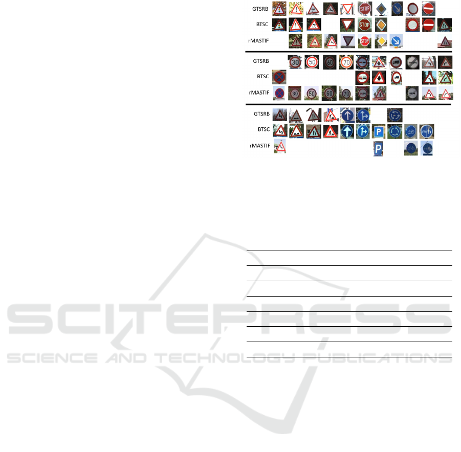
4.4 Cross-testing

To assess the generalisation ability achievable with

the different synthetic datasets we performed a test

across different countries. Our approach is to evalu-

ate a model trained in a country dataset, for instance

from Germany, in the common classes of the test set

of another country, for instance Belgium. By com-

mon classes we mean classes where the pictograms

have the same semantic meaning even though the pic-

tograms may vary slightly from country to country,

see Figure 11.

For this evaluation we selected models trained

with real data (R), synthetic with exponential bright-

ness and with solid colour backgrounds (SES). The

reason we chose the SES models is twofold: the

datasets for these models are easier to construct and

less biased since no background real imagery is re-

quired. Furthermore, these models do not have

any brightness information from the training dataset,

hence are less biased towards a particular dataset.

Essentially, from country to country, the synthetic

datasets vary in the number of classes and respective

templates.

By evaluating against test sets from other coun-

tries, we are in practice evaluating samples in differ-

ent lighting conditions, captured with different cam-

eras, and even minor differences on the sign pic-

tograms. These circumstances should be similar to

those found in a deployment of these classiﬁers in as-

sisted driving vehicles even when considering a single

country, as it is common to have multiple versions of

the same sign coexisting.

Results in Table 9 hint at a higher generalisa-

tion ability from the synthetic data when presented

with data acquired in different circumstances and/or

Figure 11: Sample signs from classes with the same seman-

tic meaning from the three datasets: GTSRB, BTSC , and

rMASTIF.

Table 9: Accuracy results for cross-testing. Each column

group describes the dataset used; Rows indicate datasets

used for evaluation purposes. Second column reports on

the number of samples from the combined test datasets.

Test set # R SER SES

Trained for GTSRB

BTSC + rMASTIF 1829 97.18 98.33 98.30

Trained for BTSC

GTSRB + rMASTIF 6410 82.39 95.75 94.73

Trained for rMASTIF

GTSRB + BTSC 8029 90.24 94.50 95.41

slightly different pictograms. The accuracy values

reported are signiﬁcantly higher for synthetic data,

and show more consistency for the different training

datasets.

4.5 Unleashing Synthetic Datasets

All previous datasets were built based only on the re-

spective training sets, i.e, all the templates used are

for trafﬁc signs that exist in the training sets, and may

therefore not be fully representative of the class. In

this section we will explore the potential of adding

further templates to cover some classes that have sig-

niﬁcant variations on the test that are not present in

the training set.

Note that in a real scenario it is perfectly legiti-

mate to gather as many templates as possible, and this

does not represent signiﬁcant additional human effort

apart from collecting the templates themselves.

Having signs that do not match exactly the sam-

ples from a particular class is a common problem in

real trafﬁc sign recognition. As mentioned before,

this can be due to the introduction of new pictograms

Bridging the Gap between Real and Synthetic Trafﬁc Sign Repositories

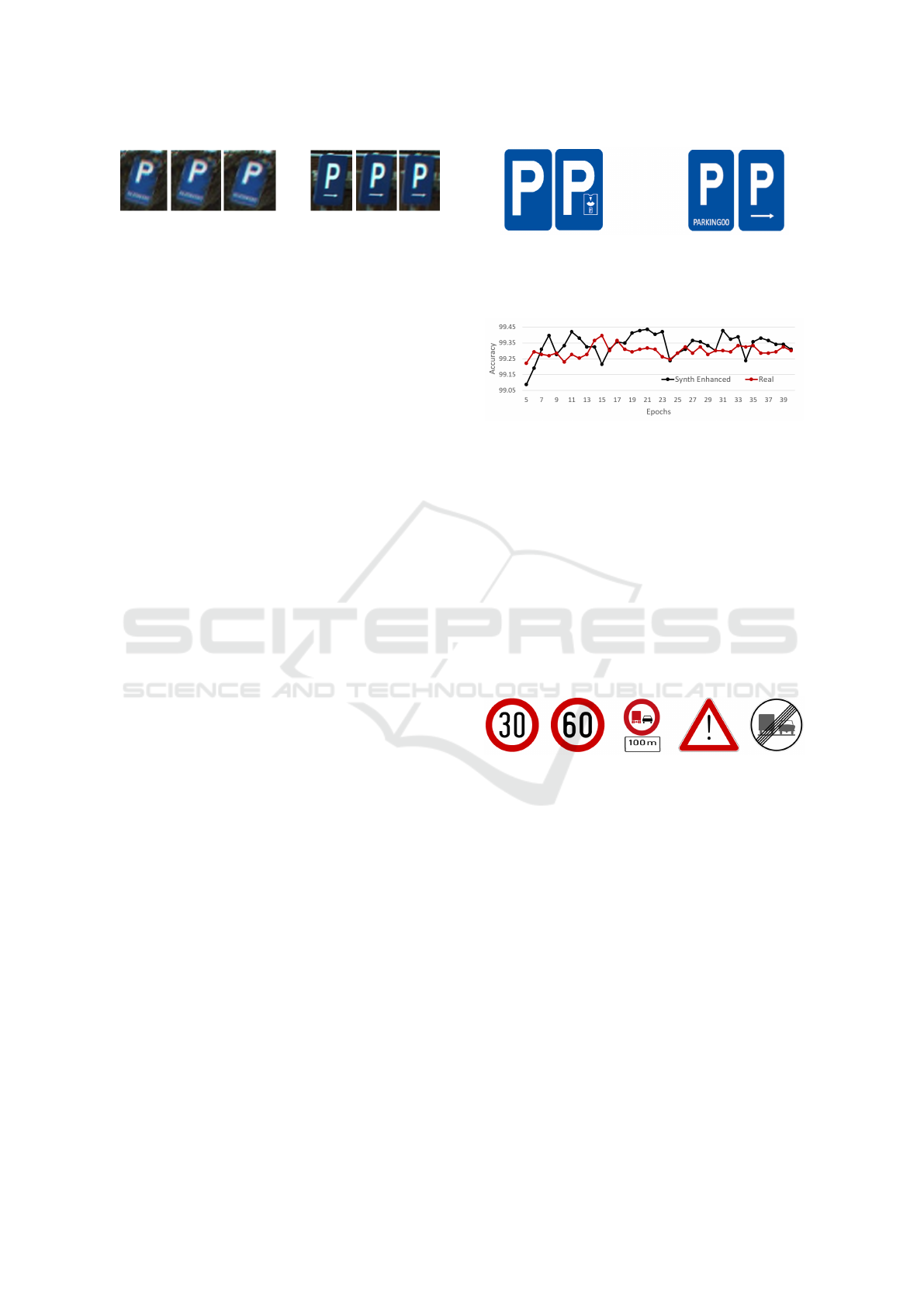
Figure 12: BTSC - Set of images misclassiﬁed by the ma-

jority of the models, both trained on real and synthetic data.

for previous classes, or different sign manufacturers.

The introduction of new signs is also a related is-

sue. When this occurs, and assuming a real data only

approach, time is required for the signs to be placed

and images captured in sufﬁcient numbers. Synthetic

signs are an excellent option to have the recognition

system dealing with these new signs from the start.

As the example shows, the only requirements are to

have the proper templates and to retrain the network.

With time, real images will become available which

can then be merged to the existing dataset, further in-

creasing the model’s accuracy.

4.5.1 BTSC

Considering the BTSC we ﬁnd a set of six images be-

longing to class 45 from the test set which are mis-

classiﬁed by the majority of the models, both trained

with synthetic and real data, see Figure 12. Since

there are no images from these trafﬁc sign variations

in the training set, the synthetic datasets previously

built did not include these templates.

Figure 13 presents the templates that can be found

in the training set (left) and the two templates that cor-

respond to the test set images in Figure 12. In BTSC

these all belong to the same class.

Five new enhanced instances of the SES datasets

were built, including the new templates for class 45

found in Figure 13. The models trained with these

datasets not only had 100% accuracy in class 45, but

also showed no adversarial effect from this addition,

surpassing the average accuracy result for the models

trained with real data.

Figure 14 presents the average test accuracy for

each epoch for both models trained with the enhanced

synthetic dataset and real dataset, showing that the en-

hanced synthetic datasets in general provided more

accurate models when compared to the real original

dataset.

We also tested merging one of these datasets with

the real BTSC dataset. After 40 epochs we got

99.76% accuracy, with only 6 misclassiﬁed images

out of 2520. This result surpasses the current state

of the art result of 99.72% reported in (Mahmoud and

Guo, 2019), with inputs that have a quarter of the pix-

els and a model with a lighter architecture. The best

epoch achieved an accuracy of 99.84%.

Figure 13: BTSC - left: templates from the training set;

right: new templates from the test set (note: the text was

added just for the template and does not correspond to any

real sign).

Figure 14: BTSC - performance comparison between mod-

els trained with the enhanced synthetic training sets vs mod-

els trained with real data.

4.5.2 GTSRB

To create the new unleashed datasets we add tem-

plates to some classes, as can be seen in Figure 15.

These templates represent variations that are either

missing from the training set or are difﬁcult to deter-

mine if they are present in the training set due to the

poor quality of some of the samples. Technically, the

it is a common combination, with this combination

being present in both the training and test sets.

Figure 15: Added templates for GTSRB.

For all the classes where new templates were

added we noticed a decrease in the number of mis-

classiﬁed samples, without relevant adverse conse-

quences in other classes. Results in Table 10 show

a signiﬁcant improvement in all synthetic models.

As in the Belgian case we also tested merging real

data with one of the SES and SJR models. The ac-

curacy obtained was 99.80% for Real + SES, and

99.79% for Real + SJR. These are marginally be-

low the state of the art results from (Haloi, 2015)

(99.81%), and our network has roughly a quarter of

the number of parameters (see Table 4), implying that

evaluation is much lighter in our case.

DeLTA 2022 - 3rd International Conference on Deep Learning Theory and Applications

Table 10: Results for unleashed GTSRB datasets.

Prev Results Unleashed

SES 99.25 ± 0.06 99.41 ± 0.08

SER 99.32 ± 0.25 99.40 ± 0.10

SJS 99.39 ± 0.08 99.50 ± 0.09

SJR 99.41 ± 0.05 99.57 ± 0.04

5 CONCLUSION

In the proposed synthetic dataset generation pipeline,

besides traditional geometric and colour operations,

we introduced Perlin and Confetti Noise as operators

to craft synthetic samples. The usage of solid colour

backgrounds, as opposed to real backgrounds, was

also explored.

In a real scenario a trafﬁc sign classiﬁer must be

able to deal with a larger number of classes than those

present in the existing datasets. Adding a new class

with real data implies gathering a signiﬁcant num-

ber of images where those signs are present, cropping

those images to obtain the ROI for the signs, and pro-

viding appropriate labels. On the other hand, with

synthetic data the addition of a new class amounts to

using a new template.

Based on the results we obtained, we strongly be-

lieve that creating synthetic datasets is an approach

worth pursuing. Using traditional methods, even

when no knowledge from real test sets was used, we

were able to clearly surpass synthetic dataset gener-

ation with previous approaches. While there is still

room for improvement, we were able to achieve re-

sults closer to real-world data with a standalone syn-

thetic training set on three distinct European test sets.

When considering merging and ensembles of real and

synthetic datasets, we surpassed previously reported

results with both real and synthetic data. Our cross

testing experiment also suggests that our synthetic

datasets provide a better generalisation ability com-

pared to real data.

As opposed to most other methods, we did not aim

at generating photo-realistic images. Yet, our results

clearly surpass previous attempts based on generat-

ing lifelike imagery, including those based on GANs.

Could this be interpreted as a hint that pursuing a sim-

ilarity with real imagery may not be the best option?

Further work is required to evaluate this.

Synthetic datasets have the potential to be able to

deal with different weather conditions such as fog,

snow and rain, as well as night time. This requires

increasing our pipeline to include these scenarios and

we expect to further explore the usage of synthetic

data in this direction.

ACKNOWLEDGEMENTS

This work has been supported by FCT – Fundac¸

para a Ci

encia e Tecnologia within the RD Units

Project Scope: UIDB/00319/2020

REFERENCES

Araar, O., Amamra, A., Abdeldaim, A., and Vitanov, I.

(2020). Trafﬁc sign recognition using a synthetic data

training approach. International Journal on Artiﬁcial

Intelligence Tools, 29.

Arcos-Garc

ıa, A., Alvarez-Garcia, J., and M. Soria-Morillo,

L. (2018). Deep neural network for trafﬁc sign recog-

nition systems: An analysis of spatial transformers

and stochastic optimisation methods. Neural Net-

works, 99.

Cires¸an, D., Meier, U., Masci, J., and Schmidhuber, J.

(2012). Multi-column deep neural network for trafﬁc

sign classiﬁcation. Neural Networks, 32:333 – 338.

Selected Papers from IJCNN 2011.

Segvic, S., Brki

c, K., Kalafati

c, Z., Stanisavljevi

c, V.,

Sevrovi

c, M., Budimir, D., and Dadi

c, I. (2010). A

computer vision assisted geoinformation inventory for

trafﬁc infrastructure. In 13th International IEEE Con-

ference on Intelligent Transportation Systems, pages

66–73.

Haloi, M. (2015). Trafﬁc sign classiﬁcation using deep

inception based convolutional networks. ArXiv,

abs/1511.02992.

Horn, D. and Houben, S. (2020). Fully automated trafﬁc

sign substitution in real-world images for large-scale

data augmentation. In 2020 IEEE Intelligent Vehicles

Symposium (IV), pages 465–471.

Jain, A., Mishra, A., Shukla, A., and Tiwari, R. (2019). A

novel genetically optimized convolutional neural net-

work for trafﬁc sign recognition: A new benchmark

on belgium and chinese trafﬁc sign datasets. Neural

Processing Letters, pages 1–25.

Juri

c, F., Filkovi

c, I., and Kalafati

c, Z. (2015). Multiple-

dataset trafﬁc sign classiﬁcation with onecnn. In 2015

3rd IAPR Asian Conference on Pattern Recognition

(ACPR), pages 614–618.

Liu, Y.-T., Chen, R.-C., and Dewi, C. (2021). Generate

realistic trafﬁc sign image using deep convolutional

generative adversarial networks. In 2021 IEEE Con-

ference on Dependable and Secure Computing (DSC),

pages 1–6.

Luo, H., Kong, Q., and Wu, F. (2018). Trafﬁc sign im-

age synthesis with generative adversarial networks.

In 2018 24th International Conference on Pattern

Recognition (ICPR), pages 2540–2545.

Mahmoud, M. A. B. and Guo, P. (2019). A novel method

for trafﬁc sign recognition based on dcgan and mlp

with pilae algorithm. IEEE Access, 7:74602–74611.

Perlin, K. (1985). An image synthesizer. SIGGRAPH Com-

put. Graph., 19(3):287–296.

Bridging the Gap between Real and Synthetic Trafﬁc Sign Repositories

Saha, S., Kamran, S. A., and Sabbir, A. S. (2018). To-

tal recall: Understanding trafﬁc signs using deep

hierarchical convolutional neural networks. CoRR,

abs/1808.10524.

Sermanet, P. and LeCun, Y. (2011). Trafﬁc sign recognition

with multi-scale convolutional networks. In The 2011

International Joint Conference on Neural Networks,

pages 2809–2813.

Spata, D., Horn, D., and Houben, S. (2019). Generation

of natural trafﬁc sign images using domain transla-

tion with cycle-consistent generative adversarial net-

works. In 2019 IEEE Intelligent Vehicles Symposium

(IV), pages 702–708.

Stallkamp, J., Schlipsing, M., Salmen, J., and Igel, C.

(2012). Man vs. computer: Benchmarking machine

learning algorithms for trafﬁc sign recognition. Neu-

ral Networks, (0):–.

Stergiou, A., Kalliatakis, G., and Chrysoulas, C. (2018).

Trafﬁc sign recognition based on synthesised training

data. Big Data and Cognitive Computing, 2(3).

Szegedy, C., Liu, W., Jia, Y., Sermanet, P., Reed, S. E.,

Anguelov, D., Erhan, D., Vanhoucke, V., and Rabi-

novich, A. (2014). Going deeper with convolutions.

CoRR, abs/1409.4842.

Timofte, R., Zimmermann, K., and Gool, L. V. (2009).

Multi-view trafﬁc sign detection, recognition, and 3d

localisation. In 2009 Workshop on Applications of

Computer Vision (WACV), pages 1–8.

Yu, F. and Koltun, V. (2016). Multi-scale context aggrega-

tion by dilated convolutions. CoRR, abs/1511.07122.

DeLTA 2022 - 3rd International Conference on Deep Learning Theory and Applications