
RoSELS: Road Surface Extraction for 3D Automotive LiDAR Point
Cloud Sequence
Dhvani Katkoria and Jaya Sreevalsan-Nair
a
Graphics-Visualization-Computing Lab (GVCL),
International Institute of Information Technology Bangalore (IIITB), Bangalore, India
Keywords:
Road Surface Extraction, 3D LiDAR Point Clouds, Automotive LiDAR, Ego-vehicle, Semantic Segmentation,
Ground Filtering, Frame Classification, Road Geometry, Sequence Data, Point Set Smoothing, Range View,
Multiscale Feature Extraction, Local Features, Global Features.
Abstract:
Road surface geometry provides information about navigable space in autonomous driving. Ground plane
estimation is done on “road” points after semantic segmentation of three-dimensional (3D) automotive Li-
DAR point clouds as a precursor to this geometry extraction. However, the actual geometry extraction is less
explored, as it is expensive to use all “road” points for mesh generation. Thus, we propose a coarser surface
approximation using road edge points. The geometry extraction for the entire sequence of a trajectory provides
the complete road geometry, from the point of view of the ego-vehicle. Thus, we propose an automated system,
RoSELS (Road Surface Extraction for LiDAR point cloud Sequence). Our novel approach involves ground
point detection and road geometry classification, i.e. frame classification, for determining the road edge points.
We use appropriate supervised and pre-trained transfer learning models, along with computational geometry
algorithms to implement the workflow. Our results on SemanticKITTI show that our extracted road surface
for the sequence is qualitatively and quantitatively close to the reference trajectory.
1 INTRODUCTION
Navigable space detection is a challenging prob-
lem in robotics and intelligent vehicle technology,
which requires an integrated solution from both com-
puter vision and computational geometry. In three-
dimensional (3D) automotive LiDAR point cloud pro-
cessing, navigable space implies the ground surface
on which a vehicle can traverse, which is predomi-
nantly the road surface. Here, the “ground” class of
points includes several fine-grained classes, namely,
“road,” “parking,” “sidewalk,” “terrain,” etc. (Paig-
war et al., 2020). The state-of-the-art methods per-
form ground point segmentation/detection followed
by ground plane estimation motivated as a precursor
to road surface extraction (Paigwar et al., 2020; Rist
et al., 2020). However, we find that ground plane es-
timation needs to be performed piecewise even for a
single point cloud, thus providing a coarse approx-
imation of the surface geometry. Piecewise estima-
tion requires systematic geometric analysis to deter-
mine the number, position, and orientation of planes
needed to jointly provide a water-tight surface. This is
a
https://orcid.org/0000-0001-6333-4161
a challenging point set processing problem, especially
as the point clouds are unstructured. Instead, we pro-
pose surface mesh extraction from the road points di-
rectly. However, generating a fine mesh with all road
points is time-consuming. This is alleviated by using
an appropriate subset of road points that sufficiently
sample the surface. Here, we propose the road edge
points and vehicle positions as this desired sample set.
Given we are using the positions of the ego-
motion of the vehicle, we can now expand the surface
extraction across all frames in a sequence. This leads
to creating a watertight road surface for the entire se-
quence, which is as seen from the point of view of
the ego-vehicle. Such a process requires all the point
clouds in the sequence, which improves the utilization
of the complete dataset.
The conventional data processing workflow for
3D automotive LiDAR point clouds involves se-
mantic segmentation, which readily detects road
points. However, the semantic segmentation results
have to be post-processed to identify curb or edge
points (Behley et al., 2021). At the same time,
ground point filtering using local height differences
is a reliable solution in the LiDAR point cloud anal-
Katkoria, D. and Sreevalsan-Nair, J.
RoSELS: Road Surface Extraction for 3D Automotive LiDAR Point Cloud Sequence.
DOI: 10.5220/0011301700003277
In Proceedings of the 3rd International Conference on Deep Learning Theory and Applications (DeLTA 2022), pages 55-67
ISBN: 978-989-758-584-5; ISSN: 2184-9277
Copyright
c
2022 by SCITEPRESS – Science and Technology Publications, Lda. All rights reserved
55

Figure 1: Summary of our proposed system, RoSELS, for
3D road surface extraction using ground points detected
from an automotive LiDAR point cloud sequence. Our sys-
tem includes two novel and significant intermediate pro-
cesses of road edge point detection and frame classification.
ysis (Arora et al., 2021). Binary clustering in point
clouds can be done here using highly statistically
significant handcrafted features, such as height dif-
ferences, to classify the points as “edge” and “non-
edge” points. Since the expectation-maximization
(EM) algorithm has been found to be effective for bi-
nary clustering of LiDAR point clouds (Kumari and
Sreevalsan-Nair, 2015), we propose a road edge point
detection method using binary clustering of ground
points. We also use the spatiotemporal locality of the
points for outlier removal to improve the ground point
detection, and thus the edge points.
Extraction of road geometry becomes challeng-
ing in the presence of turnings and complex topol-
ogy, such as crossroads. Since our work is novel
in extracting surface mesh geometry for roads, we
first focus on the workflow for straight roads. Such
a mesh generation process can be then extended to
curved roads, i.e. turnings and crossroads. Alterna-
tively, our proposed method can extract contiguous
segments of straight roads and fill the gaps between
them for short curved segments using surface correc-
tion. This solution works for most sequences with a
large fraction of contiguous straight roads. For our
requirement of identifying contiguous straight roads,
the point cloud geometry for each frame needs to be
classified. We propose a novel frame-wise point cloud
geometry classification, referred to as frame classi-
fication, using an appropriate image representation
of the geometry. We choose an intermediate image
representation specifically, as is done in state-of-the-
art deep learning classifiers for semantic segmenta-
tion (Guo et al., 2020). Here, transfer learning is used
for frame classification.
In summary (Figure 1), our proposed approach is
to detect ground points, on which both edge detec-
tion and frame classification are performed. We fur-
ther smooth the edge point set to improve the sample
set for surface mesh generation and finally extract the
road surface using geometry algorithms. Our novel
contributions are in integrating appropriate methods
in our proposed system, RoSELS (Road Surface Ex-
traction from LiDAR point cloud Sequence) for its
implementation (Figure 2). Our key contributions are:
• design and implementation of a complete auto-
mated system using ground points, for road sur-
face extraction from the ego-motion in 3D auto-
motive LiDAR point clouds,
• a novel per-frame road-geometry classification,
i.e. frame classification, using appropriate image
representation of the ground points to be used in
transfer learning.
• novel use of appropriate point set processing and
surface mesh generation methods for performing
edge point detection and road surface extraction,
respectively.
2 RELATED WORK
The source data for the design of RoSELS is the 3D
automotive LiDAR point clouds in the form of se-
quence based on the trajectory of the ego-motion of
the vehicle (Behley et al., 2019; Behley et al., 2021).
While most of the existing methods work with frame-
wise analysis, the focus here is on the entire sequence.
The state of the art in 3D automotive LiDAR point
cloud processing on the following topics is relevant
to our work:
Ground Point Segmentation: Our starting point for
detecting road edge points is ground point segmen-
tation, which is equivalent to point-wise classification
into “ground” and “non-ground points.” This has been
an active area of research since the mid-2000s (Paig-
war et al., 2020; Arora et al., 2021). There are
two parallel approaches – (i) use height-based hand-
crafted features and traditional machine learning, and
(ii) use convolutional neural networks (CNNs) or con-
volutional encoder-decoder, either with image repre-
sentation for its projection (e.g. sparse pseudo image,
bird’s eye view (BEV), range image, etc.) or with
3D points directly (Guo et al., 2020). The latter can
be directly used for binary road segmentation (Gigli
et al., 2020), specifically. While CNNs work the best
for trained environments, they are not as generalized
for other environments and are expensive for train-
DeLTA 2022 - 3rd International Conference on Deep Learning Theory and Applications
56

Figure 2: (Left) Our proposed workflow of RoSELS, for generating 3D road surface, from input 3D LiDAR frame-wise point
clouds in a sequence and its trajectory information (position and pose of the vehicle). Our workflow is structured and proceeds
from point-, frame-, to sequence-wise processing. (Right) Frame classification implemented on top-view images of ground
points in each frame, using (i) transfer learning using ResNet-50 architecture (He et al., 2016). The possible class hierarchy
for frames is given in (ii), of which we currently focus on the first level of straight and curved road classes.
ing. However, depending on the requirement, height-
based feature extraction has been still used for ground
point segmentation (Arora et al., 2021; Ouyang et al.,
2021). For instance, either geometry-based filter-
ing (Ouyang et al., 2021) or processing of elevation
map image (Shen et al., 2021) is done. Such images
at various resolutions serve as input to an ensemble
edge detection for probabilistic ground point segmen-
tation, through voting (Arora et al., 2021).
An alternative method is the fine-grained multi-
class semantic segmentation (Guo et al., 2020), where
the appropriate classes can be functionally combined
as “ground” class (Paigwar et al., 2020; Arora et al.,
2021; Shen et al., 2021). Projection-based methods
using deep learning form a widely used class of se-
mantic segmentation methods, for which range im-
ages are extensively used (Milioto et al., 2019; Cort-
inhal et al., 2021). Another set of networks directly
use 3D point sample sets, e.g. RandLA-Net (Hu et al.,
2020), SCSSnet (Rist et al., 2020), etc.
RoSELS uses the lower-cost ground segmentation
solution using supervised learning with hand-crafted
features, as our goal is to identify the road edge points
using the ground segmentation.
Road Edge Extraction: Curb extraction has been
studied for mobile laser scanning (MLS)/LiDAR
point clouds (Zhao et al., 2021; Sui et al., 2021),
monocular images acquired by moving vehicle (Stain-
vas and Buda, 2014), and elevation map from 2D laser
scanner (Liu et al., 2013). All of these methods in-
volve identifying candidate points or positions using
elevation filtering and using appropriate line fitting al-
gorithms. Our work is closest to road boundary ex-
traction for MLS point clouds (Sui et al., 2021) where
the edge points are located by searching outwards
from the vehicle trajectory. The difference, however,
is that for the MLS point clouds, the search is per-
formed in the candidate point set, and we exploit the
range image view of the vehicle LiDAR point cloud,
on which the search is performed.
In the benchmark SemanticKITTI dataset for ve-
hicle LiDAR point clouds, the curb points are labeled
as “sidewalk,” where the points are first labeled in
tiles by human annotators (Behley et al., 2019), and
the road boundary/curb points are then specifically re-
fined (Behley et al., 2021). In the baseline approaches
in the benchmark test of semantic segmentation im-
plemented using deep learning architectures, the IoU
(intersection over union) score for sidewalk is 75.2%
with RangeNet++ (Milioto et al., 2019) and 75.5% in
SCSSnet (Rist et al., 2020), which is relatively low.
Thus, we observe that the deep learning solutions
for semantic segmentation cater well to classifying
road points, but have a gap in road edge point de-
tection. This can be explained by the class imbal-
ance. Hence, we propose a structure-aware method
for road edge detection from ground points. Our
approach is to detect road edge points using the
height-based handcrafted features in supervised learn-
ing methods (Arora et al., 2021).
Scene Classification: We look at the state of the
art in scene classification, which is the closest to our
novel frame classification. Coarse scene classifica-
tion has been done on satellite or aerial images using
transfer learning (Zhou et al., 2018b), where ResNet
(Residual Network) (He et al., 2016) has demon-
strated near-accurate performance. ResNet with 50
layers (ResNet-50) is optimal in performance and cost
for land-cover classification of remote sensing im-
ages (Scott et al., 2017). Road type classification
based on its functionality as “highway,” and “non-
highway,” has been done on the KITTI vision bench-
mark suite using AlexNet (Krizhevsky et al., 2012).
Since ResNet-50 has worked better on aerial images,
we choose to use the same in RoSELS instead of
AlexNet, as we require a deep learning architecture
that works best for the top-view of the road. The top-
views perceptually show a clear distinction between
RoSELS: Road Surface Extraction for 3D Automotive LiDAR Point Cloud Sequence
57

different road geometry classes, namely the “straight”
and “curved” roads.
Ground Plane Estimation: Recent work on road
extraction has considered the ground plane estimation
and segmentation to be a precursor to the geometry
extraction (Paigwar et al., 2020; Rist et al., 2020).
GndNet uses 2D voxelization or pillars to generate
a pseudo-image which then is passed on to a con-
volutional encoder-decoder to estimate ground eleva-
tion (Paigwar et al., 2020). SCSSnet uses semantic
segmentation to identify ground points and performs a
simple ground plane estimate (Rist et al., 2020). Since
our goal is to perform coarse geometry extraction di-
rectly, we identify edge points and triangulate them
along with trajectory points. RoSELS is also differ-
ent from the mesh map, which is a triangulation of an
automotive LiDAR point cloud using surface normals
derived from range images (Chen et al., 2021).
3 PROPOSED WORKFLOW &
IMPLEMENTATION
We propose a novel workflow to extract approxi-
mate road geometry, for straight roads. The work-
flow of RoSELS consists of five key steps, namely,
(S
1
) ground point detection, (S
2a
) frame classification
implicitly giving the road geometry, (S
2b
) road edge
point detection, (S
3
) edge point set smoothing, and
(S
4
) 3D road surface extraction. As shown in Fig-
ures 1 and 2:
• S
1
is a point-wise operation, i.e. it is implemented
on each point in the point cloud, i.e. a frame.
• The frame-wise operations, S
2a
and S
2b
, are de-
coupled and implemented in parallel.
• S
3
and S
4
are sequence-wise operations, and
hence requires the trajectory information of the
vehicle for the entire sequence.
The overall workflow of RoSELS, i.e. S
1
to S
4
, is
captured in Algorithm 1. The partial workflows
of the point-wise classification process (S
1
) and the
sequence-wise road edge extraction (S
2a
, S
2b
, S
3
) are
given in Algorithms 2 and 3, respectively. Our pro-
posed road surface extraction gives the surface as vis-
ible from the point-of-view of the vehicle. Hence, the
vehicle is called an ego-vehicle (Rist et al., 2020).
S
1
– Ground Point Detection: The point cloud is
classified into “ground” and “non-ground” points for
ground point detection, for which the motivation is
explained in Section 2. S
1
involves two sequential
substeps, namely, outlier removal and semantic seg-
mentation. Here, we exploit the temporal and spatial
locality of the points.
Outlier Removal – Point cloud registration or scan
matching, which is widely implemented using the It-
erative Closest Point (ICP) registration (Besl Paul and
McKay, 1992), is performed on two different point
clouds to find the correspondence pairs of points be-
tween the two. A correspondence pair implies that
there exists an affine transformation (e.g., scaling, ro-
tation and translation) to make a point in one cloud
equivalent to a point in the other cloud.
The registration uses temporal locality, i.e. points
in a frame must be preserved in consecutive frames.
Thus, we find correspondence pairs of points in con-
secutive frames and mark the remaining points as
“outliers” to be filtered out. Owing to the continu-
ity of motion across frames, iterative registration on
three consecutive frames is implemented at a time.
For a given current frame x, we perform registration
in two steps. In the first step, outliers are removed
in frame (x − 1), using registration between frames
(x−1) and (x −2). Then, the same process is repeated
on frame (x), after performing registration between
(x) and (x − 1).
Semantic Segmentation – Many of the objects cor-
responding to non-ground points have elevation (z)
higher than that of the ground. Hence, height-based
features are best suited for differentiating ground
points from others (Arora et al., 2021). The “ground”
class is a combination of several fine-grained seman-
tic classes pertaining to the ground, thus making it a
coarser class. We extract the local and global spatial
handcrafted features, and use them in Random For-
est Classifier (RFC) (Breiman, 2001) to segment the
point cloud to the ground and the non-ground classes.
The feature extraction is implemented on the point
cloud in each frame, after outlier removal. Here, we
compute multi-scale local height features, for three
scales. Multi-scale features, i.e. features captured at
different spatial resolutions, are known to work bet-
ter than a single scale for LiDAR point classifica-
tion using RFC (Weinmann et al., 2014). Here, for
each point, we select a hybrid neighborhood search
that combines the criteria of the spherical and the k-
nearest neighborhoods (knn). Thus, we identify at
most k-nearest neighbors (knn) of a point that are
within a given distance, r, from the point. The height
features used for ground point detection are listed in
Table 1. These extracted features are computed and
used in an RFC for both training and testing.
S
2a
– Road Edge Point Detection: The points on
the road edges are those ground points that physically
interface with the curb/sidewalk (Behley et al., 2021).
RoSELS requires extraction of both the left and right
banks of the road. Edge detection is a well-studied
problem in image processing, where gradient infor-
DeLTA 2022 - 3rd International Conference on Deep Learning Theory and Applications
58

Table 1: Point-wise features at each scale for ground detec-
tion (S
1
).
Local Features Global Features Global Features
Point-based Frame-based
Height-based
– Difference from max.
– Difference from mean
– Standard deviation
Height-based
– Value (z-coordinate)
– Difference from mean
(of frame)
Position-based
– Distance from sensor
– Elevation angle θ
Height-based
– Difference from mean
– Standard deviation
mation is used for identifying the edges in images and
is implemented using the widely used three-step pro-
cess, which includes differentiation, smoothing, and
labeling (Ziou and Tabbone, 1998). Applying the
same approach as in image processing, the height gra-
dient is used as the characteristic feature to identify
the points on road edges.
However, our method of road edge detection is
different from the edge detection in images in two
salient ways. Firstly, smoothing is needed for only
road edge points, and not the entire point cloud, unlike
the image smoothing done for edge detection in im-
ages. Thus, we perform edge smoothing and labeling
steps, which are now jointly referred to as edge point
set smoothing, on ground points. Secondly, in our
case, the road extraction depends on the road geome-
try information, i.e. determined during S
2b
. Addition-
ally, unlike the differentiation step which is done on a
frame, the edge point set smoothing (i.e. S
3
) requires
the information of the sequence trajectory for coor-
dinate system transformation. Thus, the three steps
do not follow successively, here. Thus, S
2a
is exclu-
sively for the differentiation step, and edge point set
smoothing and labeling are implemented in S
3
.
Height Gradient-based Differentiation – Here, the
first-order derivatives or gradients of height values are
computed exclusively of the ground points. We pro-
pose point clustering for this task with two specific
requirements. Firstly, we cluster road points into re-
gions with low and high height-gradient, referred to as
“flat” and “non-flat” regions, respectively. Secondly,
the features needed for clustering are computed using
height differences. Of the hand-crafted features used
for semantic segmentation of 3D airborne and terres-
trial LiDAR point clouds (Weinmann et al., 2014), we
choose the two appropriate height-difference (∆
z
) fea-
tures, namely, in a local neighborhood, and in the 2D
accumulation map. The 2D accumulation map gen-
erates local neighborhoods of points projected to xy-
plane, within a square of fixed length (e.g. 0.25m),
centered at the point. For the clustering process, we
observe that the clear clusters do not exist in vehicle
LiDAR point clouds. The Expectation-maximization
(EM) algorithm (Dempster et al., 1977) has been
known to work better than the k-means clustering in
such scenarios. The EM algorithm works with an un-
derlying assumption of the existence of a Gaussian
Mixture Model (GMM) in the data. Thus, assuming
a bimodal data distribution in the 2D feature space,
we use the EM algorithm to determine two clusters of
points belonging to the flat and non-flat regions.
Projection to Range Images – The edge points fall in
the non-flat regions, where those closest to the cen-
terline, i.e. the trajectory, are the desired ones. For
a frame-wise operation of centerline detection, the
range image of the frame is the best representation of
the frame to use. The centerline is defined as the col-
umn of the range image where the sensor, i.e. the ego-
vehicle, is positioned. A range image is a dense ras-
terized representation of the occluded view from the
ego-vehicle point. Thus, it is generated as the spheri-
cal projection of the points nearest to the ego-vehicle,
and the pixels are colored based on the attribute of
the nearest point in the pixel. The image resolution
is given by the angular resolution in the elevation and
azimuthal angles. For instance, the angular resolu-
tion for the Velodyne HDL-64E S2
1
that was used for
SemanticKITTI data (Behley et al., 2019) acquisition
has 64 angular subdivisions (i.e. ≈0.4
o
) in elevation
angle spanning for 26.8
o
, and similarly 0.08
o
angu-
lar resolution for 360
o
azimuthal angle, which gives a
64 × 4500 resolution of range images.
Edge Detection – In order to determine the edge
points, we propose the use of a scanline algorithm
on the range image. We first scan the image of size
H ×W row-wise, where the key positions relative to
the ego-vehicle, in the pixel space, are:
• at P
c f
, i.e. (0,
W
2
), which indicates the centerline
column in the front;
• at P
cbL
, i.e. (0, 0), which indicates the centerline
column in the back (rear), but on the left-side of
the ego-vehicle; and
• at P
cbR
, i.e. (0,W), which indicates the centerline
column in the back, but on the right-side.
Note that the left and right sides of the ego-vehicle
are with respect to its front face. Thus, at each row,
the pixels on the centerline columns are used as the
reference for scanning the pixels in the row in the ap-
propriate direction, until a pixel containing a non-flat
region point is encountered. For front left and right
pixels for non-flat region points, we traverse from P
c f
towards P
cbL
and P
cbR
, respectively. Similarly, in the
rear side, for left side, we traverse from P
cbL
to P
c f
,
and for right side, from P
cbR
to P
c f
. After locating
these pixels, their corresponding 3D LiDAR points
are to be determined. We refer to these row-wise
1
This information is from the sensor specification sheet
as published by the sensor manufacturer.
RoSELS: Road Surface Extraction for 3D Automotive LiDAR Point Cloud Sequence
59

points as p
f L
, p
bL
on the left side, and p
f R
, p
bR
on the
right side. These points are added to the side-specific
sets, EP
L
and EP
R
, for the left and right sides, respec-
tively in each frame.
In this step, the height differences pertaining to
other surface variations on the road, e.g. potholes, are
disregarded. We visualize the points in EP
L
and EP
R
and ensure that the edges of other surface artifacts are
not labeled as road edge points. This is significant, as
the artifact points would adversely impact the perfor-
mance of RoSELS.
S
2b
– Frame Classification: The underlying road
geometry influences the surface extraction method, as
expected. Our proposed approach uses the road edge
points for generating triangulated (surface) meshes.
The edge points along the road boundary are to
be sampled sufficiently for accurate edge extraction.
This sampling is dependent on the road curvature.
We first consider a broad classification of
“straight” and “curved” roads (Figure 2, (Right)(ii)).
We restrict our current work to straight roads for three
reasons. Firstly, curved roads need more samples as
edge points so that the edges can be extracted with
sufficient accuracy, and the sample size is determined
using geometric methods. Secondly, to extract the
curved road edges piecewise, the larger road topol-
ogy is not sufficiently captured from the point of view
of the ego-vehicle. The road topology for turnings
and crossroads involve T- and X-intersections which
need to be captured, that is beyond the scope of the
current workflow. Thirdly, additional interior road
points are needed to extract curved road surfaces ap-
propriately. Addressing these three issues requires an
in-depth study which is beyond the scope of our cur-
rent work. Hence, we show a proof-of-concept for our
workflow for straight roads exclusively.
Transfer Learning using ResNet-50 Architecture –
For 3D LiDAR point cloud sequence, we observe that
each frame distinctly demonstrates the road geometry
from its top-view, i.e. 2D projection of the points on
the x-y plane. To exploit the perceptual differences
between frames, we propose the use of transfer learn-
ing using ResNet-50. It has been used for an effec-
tive scene classification of perceptually distinguish-
able images (He et al., 2016).
The attribute values of the points are used to
render the 2D top-view RGB image using percep-
tually uniform sequential colormap, i.e. the viridis
colormap. The sequential colormap is further dis-
cretized to a predetermined number of bins, say 5
bins. The ground points detected in S
1
are ren-
dered using the colormap with respect to their remis-
sion values. We implement transfer learning with the
ResNet50 model on these images (Figure 2(Right)).
Here, pre-trained weights for image classification of
ImageNet are used, as per the de facto standard in
transfer learning on images.
S
3
– Edge Point Set Smoothing: Now, the road edge
points identified in S
2a
are fitted to form edges. These
edges are smoothed owing to the noise in the edges.
The smoothing is done separately for the left and right
sides of the road to avoid filtering out relevant points.
Edge labeling refers to the localization of edges and
filtering out false positives. Thus, S
3
includes both
smoothing and labeling. The edge processing is im-
plemented in the world coordinate system which con-
tains the entire trajectory of the sequence. Hence, the
first substep is the coordinate system transformation.
Local to World Coordinate System Transformation
– This transformation ensures that the smoothed
edge exists as-is in the 3D world space. Also, the
smoothing and transformation operations are non-
commutative, i.e. the order of their implementation
has to be strictly maintained. Hence, we now add
the trajectory information as an input to the work-
flow (Figure 2(Left)). This input contains the posi-
tion and poses of the ego-vehicle at each frame of the
sequence. The change in position and pose is repre-
sented as transformation matrices. These matrices are
applied on the edge points in each frame to transform
them to the 3D world space.
Point Set Smoothing and Labeling – The straight
road edges are smoothed using the transformed co-
ordinates. We first determine subsequences of frames
that form contiguous segments of straight roads. This
is implemented separately for the left and right sides.
The random sample consensus (RANSAC) line fit-
ting model (Fischler and Bolles, 1981) is applied to
each such subsequence. Thus, we get disconnected
smooth line segments, that look like dashed lines, on
both sides of the road.
S
4
– 3D Road Surface Extraction: After smooth-
ing, the road surface is extracted as a triangulated
mesh formed with the left and right edge points for
each contiguous segment of the straight road. Here, a
constrained Delaunay tetrahedralization (Shewchuk,
2002) is implemented and is followed by the extrac-
tion of the outer/external surface of the tetrahedral
mesh. This generates better quality triangles com-
pared to performing 2D Delaunay triangulation on
projections of the 3D points.
Implementation of RoSELS: The RoSELS has been
implemented on Intel core i7 CPU with 12 GB of
RAM. We have used Open3D library APIs (Zhou
et al., 2018a) for point cloud registration in S
1
. For
neighborhood computation in S
1
and S
3
, Open3D
KDTree has been used. The scikit-learn library
APIs (Buitinck et al., 2013) have been used for im-
DeLTA 2022 - 3rd International Conference on Deep Learning Theory and Applications
60

Input : A sequence S of frame-wise point clouds
{P( f
i
) : 0 ≤ i < n
f rames
} with frame f
i
at
index i
Input : Trajectory information of the sequence
T (S)
Output: 3D surface mesh of the extracted road R
m
P
edge
← {} // Set of edge points in S
for frame f in S do
// Ground point detection
// using Algorithm 2
G
p
( f ) ← ground-point-detection(P( f ))
// Frame classification using
// top-view image as straight- or
// curved-road
TV
img
( f ) ← projection-xy-plane(G
p
( f ))
road type( f ) ←
classify-using-transfer-learning(TV
img
( f ))
// Straight-road edge detection
// using Algorithm 3
if road type( f ) is “straight-road” then
E
p
( f ) ←
straight-road-edge-detection(G
p
( f ))
P
edge
← P
edge
∪ E
p
( f ) // Merging all
// edge points
end
end
R
m
← generate-triangulated-mesh(P
edge
)
return R
m
Algorithm 1: The complete workflow of RoSELS for
road surface extraction from a sequence.
plementing the RFC and GMM models in S
1
and S
2a
,
respectively. Frame classification model in S
2b
has
been implemented using Keras APIs (Chollet et al.,
2015) and the model has been trained for five epochs.
Edge point set smoothing in S
3
has used the RANSAC
model from the scikit-image library. PyVista library
APIs (Sullivan and Kaszynski, 2019) has been used
for geometry computation in S
4
.
4 EXPERIMENTS & RESULTS
RoSELS specifically requires an input dataset that has
sequence(s) of LiDAR point clouds through a trajec-
tory of the vehicle, and also, sufficient annotations for
generating machine learning solutions. In that regard,
SemanticKITTI (Behley et al., 2019) serves well as
our test data.
Input : Point cloud P( f ) at a frame f
Output: Set of ground points G
p
( f )
G
p
( f ) ← {} // Set of ground points
for point p in point cloud P( f ) do
// Extraction of all features,
// as given in Table 1
for 0 ≤ i < n
scales
do
N
i
← find-local-neighborhood(p,
neighborhood size)
end
F
p
← compute-features (P
i
, N
1
, . . ., N
n
scales
)
// Classification of points as
// ground or non-ground points
type(p) ←
classify-using-Random-Forest-Classifier(F
p
)
// Add ground points to the output
if type(p) is “ground” then
G
p
( f ) ← G
p
( f ) ∪ {p}
end
end
return G
p
( f )
Algorithm 2: Ground point detection per frame,
i.e. S
1
.
4.1 Dataset
The SemanticKITTI dataset (Behley et al., 2019) has
been published primarily for three benchmark tasks,
namely semantic segmentation and scene comple-
tion of point clouds using single and multi-temporal
scans. Since our work is different from the bench-
mark tasks, validation is not readily available for the
dataset. Given its fit as input to RoSELS, we use Se-
manticKITTI for our experiments and provide an ap-
propriate qualitative and quantitative assessment.
The SemanticKITTI dataset comprises of over
43,000 scans of which over 21,000 are from the train-
ing sequence IDs, 00 to 10. We have used the se-
quence 08 as the validation/test set, as prescribed by
the data providers, thus training our model on the re-
maining training sequences for our classifier models,
i.e. RFC model for ground point detection (S
1
), and
transfer learning model for frame classification (S
2b
).
We have only used every 10
th
frame of training se-
quences of SemanticKITTI since frames are captured
in 0.1s and our subsampling ensures significant varia-
tions in the vehicle environment are captured without
incurring high computational costs. We have found
that including more overlapping data resulted in in-
creased computation without adding new information.
Overall, the dataset has annotations for 28 dis-
tinct classes for the semantic segmentation bench-
mark task. We consider five such classes, namely
RoSELS: Road Surface Extraction for 3D Automotive LiDAR Point Cloud Sequence
61

Input : Set of ground points G
p
( f ) at a frame f with label “straight-road”
Input : Trajectory information of the sequence T(S)
Output: Set of road edge points E
p
( f )
NF
p
( f ) ← {} // Set of non-flat region points
for point p in G
p
( f ) do
A
m
← compute-accumulation-map(p)
N
g
← find-local-neighborhood(p, neighborhood size)
F
∆z
← compute-local-height-difference-features(G
p
, N
g
, A
m
)
region type(p) ← classify-using-GMM(F
∆z
) // Classify as flat or non-flat region
if region type(p) is “non-flat” then
NF
p
( f ) ← NF
p
( f ) ∪ {p}
end
end
// Generate range image of size (H,W ) using non-flat region points
R
img
( f ) ← range-image-generation(NF
p
( f ), G
p
( f ), H,W )
EP
L
← {}
EP
R
← {}
// Detect edge points from range image
for 0 ≤ row < H do
P
c f
← (row,
W
2
) // Determine centerline pixel in the front side
// using the column for sensor
P
cbL
, P
cbR
← (row, 0), (row,W ) // Determine centerline pixel in the back (rear) side
// using the columns for sensor
p
f L
← point-in-pixel-furthest-from-centerline-in-pixel-interval(P
c f
,
P
c f
, P
cbL
)
p
f R
← point-in-pixel-furthest-from-centerline-in-pixel-interval(P
c f
,
P
c f
, P
cbR
)
p
bL
← point-in-pixel-furthest-from-centerline-in-pixel-interval(P
CRL
,
P
cbL
, P
c f
)
p
bR
← point-in-pixel-furthest-from-centerline-in-pixel-interval(P
CRR
,
P
cbR
, P
c f
)
EP
L
← EP
L
∪ {p
f L
, p
bL
}
EP
R
← EP
R
∪ {p
f R
, p
bR
}
// Correct the selected edge points in 3D world space
for point p in {p
f L
, p
f R
, p
bL
, p
bR
} do
p ← transform-using-trajectory-information(p, T (S))
end
end
// Postprocessing edges to remove outliers
EP
L
← smooth-edge-using-RANSAC-line-fitting(EP
L
)
EP
R
← smooth-edge-using-RANSAC-line-fitting(EP
R
)
E
p
( f ) ← EP
L
∪ EP
R
return E
p
( f )
Algorithm 3: Straight road edge detection per frame, followed by collation of edge points from all frames (S
2a
,
S
2b
, S
3
).
“road,” “parking,” “sidewalk,” “other ground,” and
“terrain,” together as the “ground” class in RoSELS.
Thus, the “non-ground” class implies the remaining
classes, i.e. movable objects, such as “car,” “bicy-
cle,” etc., and stationary objects, such as, “building,”
“fence,” “vegetation,” etc. The curbs of the road are
labeled as sidewalk (Behley et al., 2021) and are im-
portant in our evaluation.
For the frame classification, we have manually an-
notated all frames in all training sequences, i.e. from
00 to 10, into “straight,” “crossroad,” and “turning.”
4.2 Parameter Setting and Experiments
For multi-scale feature extraction for ground point
detection using RFC, hybrid criteria for neighbor-
hood determination have been used for three differ-
ent scales. We have commonly used the constraint
of r of 1m for the spherical neighborhood in all the
scales, and variable k values for the knn neighbor-
hood, i.e. k = 50, 100, 200 neighbors. We have sys-
tematically experimented with several combinations
of neighborhood criteria to arrive at this parameter
DeLTA 2022 - 3rd International Conference on Deep Learning Theory and Applications
62
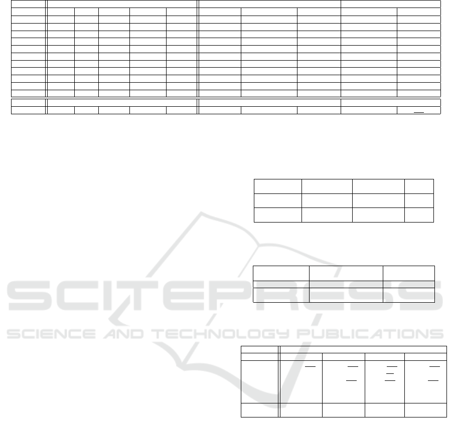
Table 2: Specifications of the SemanticKITTI sequences used for training and validation/testing in RoSELS.
Seq. ID # Frames Ground truth (GT) Filtered after outlier removal in S
1
Training Total Used Straight Crossroad Turning # Points # “Ground” points “Road”
*
(%) # “Ground” points “Road”
*
(%)
00 4,541 455 238 205 12 55,300,603 21,242,723 45.2 20,928,740 45.2
01 1,101 111 69 23 19 11,737,924 6,684,753 71.8 6,425,398 72.0
02 4,661 467 195 134 138 58,678,800 26,955,344 42.8 26,568,086 42.8
03 801 81 17 48 16 10,038,550 4,563,802 48.8 4,485,650 49.0
04 271 28 25 3 0 3,518,075 1,816,228 65.9 1,779,528 66.4
05 2,761 277 172 102 3 34,624,816 14,025,815 40.5 13,802,511 40.5
06 1,101 111 54 57 0 13,567,503 8,417,991 34.1 8,223,230 34.1
07 1,101 111 54 57 0 1,3466,390 5,301,837 48.1 5,233,937 48.2
09 1,591 160 42 39 79 19,894,193 9,313,682 45.0 9,159,419 45.1
10 1,201 121 64 32 25 15,366,254 5,608,339 43.7 5,487,403 43.9
All 19130 1922 930 700 292 236,193,108 103,930,514 45.3 102,093,902 45.3
Testing Filtered and Classified in S
1
08 4071 408 261 124 23 50,006,369 21,943,921 40.3 20,919,150 41.1
*
Our annotation of “ground” combines five classes, namely, “road,” “parking,” “sidewalk,” “terrain,” and “other ground,” as given in SemanticKITTI dataset. Percentage values in
columns 9 and 11 give the fraction of ground points in columns 8 and 10, respectively, that are annotated as “Road” in SK. Boldface indicates improvement in retaining road points, thus
demonstrating the efficiency of processes in S
1
.
setting. Similarly, we have used similar hybrid cri-
teria, i.e. r = 1m and k = 50 for finding the local
neighborhood of ground points for computing height-
difference features to be used in the GMM for detect-
ing flat and non-flat regions.
We have used sequences 01, 05, 07, and 08 from
the training dataset for road surface extraction. We
have also tested our proposed method on sequence 15
from the test dataset. Our results for all the sequences
are given in Figure 3. The performance of our edge
point set smoothing in S
3
in sequence 07 is demon-
strated in Figure 4.
4.3 Results
For each step in our workflow, we perform both qual-
itative analysis using visualization and appropriate
quantitative evaluation.
S
1
: Ground Detection: The details of the sequences
used in our models are given in Table 2. For all train-
ing sequences, we observe that the percentage of road
points preserved as ground points does not reduce af-
ter outlier removal in S
1
. This shows the efficiency
of our outlier removal process while preserving the
“road” points. The results of our ground detection
using RFC and different experiments we performed
by including multi-scale features and registrations are
given in Table 3. The table shows the average ac-
curacy and the mean IoU (mIoU) for ground class
across all frames of test sequence 08. We observe that
GndNet (Paigwar et al., 2020) has reported an mIoU
of 83.6%, but is not comparable here, as their mIoU
has been calculated across both the ground and non-
ground classes together. Similarly, ground segmenta-
tion in (Arora et al., 2021) has reported an mIoU for
the “ground” class as 78.46% but it is not compara-
ble as their “ground” class includes “vegetation” ad-
ditionally. While we cannot directly compare, these
mIoU scores indicate that our approach for ground
point classification shows a considerably high level
Table 3: Ground detection using random forest classifier
(RFC).
Set of points # Scales Classification mIoU
to be classified for local features accuracy (%-age) (%-age)
All points
1 (single scale) 96.37 89.38
3 (multi-scale) 96.63 90.63
Filtered
*
points
1 (single scale) 96.58 89.47
3 (multi-scale) 96.91 90.79
* Filtered points are those that were retained after outlier removal in S
1
.
Table 4: Results of frame classification using transfer learn-
ing.
#Class hierarchy
*
Class outcomes Classification
levels accuracy (%age)
1 Straight road, Curved road 82.35
2 Straight road, Crossroad, 78.51
Turning
* Frame class hierarchy is as shown in Figure 2(Right,(ii)).
Table 5: Class distribution of road edge points in extracted
surface.
GT Class ↓ # Points (% age)
Seq. ID → 01 05 07 08
Road 12,437 (94.0) 10,093 (63.4) 3,864 (76.5) 19,856 (84.3)
Parking 0 408 (2.6) 448 (8.9) 710 (3.0)
Sidewalk 6 (0.0) 5,243 (32.9) 695 (13.8) 2,599 (11.0)
Terrain 519 (3.9) 161 (1.0) 42 (0.8) 393 (1.7)
Other-
ground 276 (2.1) 18 (0.1) 0 0
Non-
ground 0 0 0 7 (0.0)
* Underlined %-age values show that road edge points in the extracted surface belong to
“road” and “sidewalk” classes, predominantly, and as desired.
of accuracy.
S
2a
: Frame Classification: As an experiment, we
have trained two different frame classification mod-
els corresponding to the different levels of frame/road
geometry class hierarchy (Figure 2, (Right)(ii)). The
first model is for classification into straight or curved
roads, and the second one is for classification into
straight roads, crossroads, and turnings. The vali-
dation accuracy on sequence 08 for both the frame
classification models is shown in Table 5. Given the
higher accuracy at the first level of classification, we
have used the model for “straight” and “curved” roads
here. These accuracy results can be further improved
in future work by addressing the class imbalance in
both hierarchical levels (Table 2).
RoSELS: Road Surface Extraction for 3D Automotive LiDAR Point Cloud Sequence
63
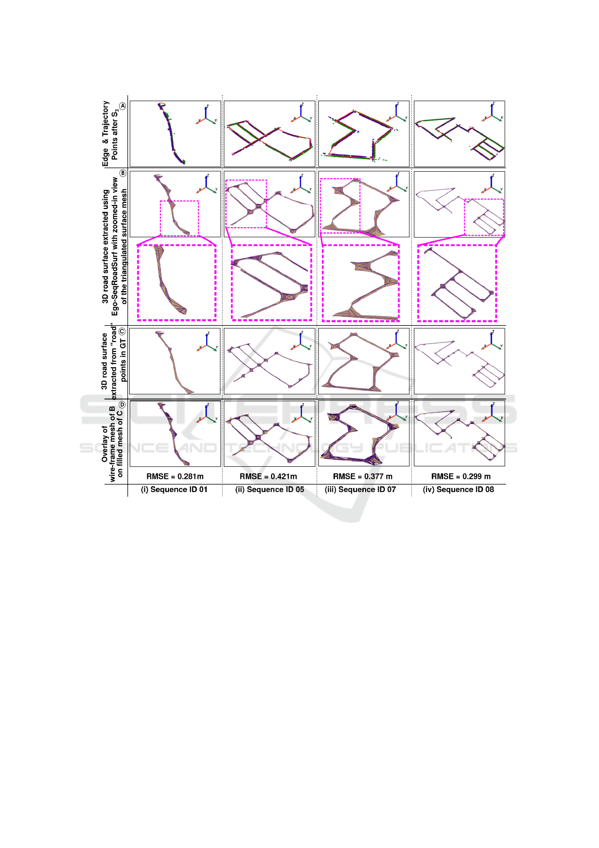
Figure 3: Results of implementing RoSELS on training sequences of SemanticKITTI (Behley et al., 2019), where 01, 05,
and 07 have been used for training our learning models, and 08 has been used for validation/testing. Row A follows the color
scheme as mentioned in Figure 4. For rows B, C, and D wireframe meshes are shown in indigo and filled meshes are shown
in tan color.
S
3
: Edge Point Set Smoothing: The class distri-
bution of our road edge points after S
3
is shown in
Table 5. We observe that most of the edge points be-
long to the “road” class predominantly, followed by
the “sidewalk” class. This shows that our approach
identifies edge points that are annotated as “road” or
“sidewalk,” as expected. This shows the combined
efficiency of S
2a
, S
2b
, and S
3
. The edge point set
smoothing results for sequence 07 in Figure 4 show
that the noise in edge points is substantially reduced,
thus giving smooth road edges on the left and right of
the trajectory.
To quantify the error, we perform these three steps
on the “road” points in the ground truth (GT), and
compute the root mean square error between the edge
point sets computed using “road” (GT) and “ground”
(detected in S
1
) points. We perform this analysis ow-
ing to the absence of ground truth of edge points and
extracted surface. The RMSE values for sequences
01, 05, 07, and 08 are given in Figure 3. Given that
each frame has an extent of 51.2m in front of the ve-
hicle and 25.6m on either side (Behley et al., 2019),
we observe that the RMSE errors are relatively low.
S
4
: 3D Road Surface Extraction: The results of
the 3D extracted surface for trajectories of different
sequences are visualized in Figure 3. Our qualita-
tive results show that RoSELS works efficiently on
straight paths, closed trajectories, and complex trajec-
tories that predominantly have large contiguous seg-
ments of straight roads. Our results of surfaces ex-
DeLTA 2022 - 3rd International Conference on Deep Learning Theory and Applications
64
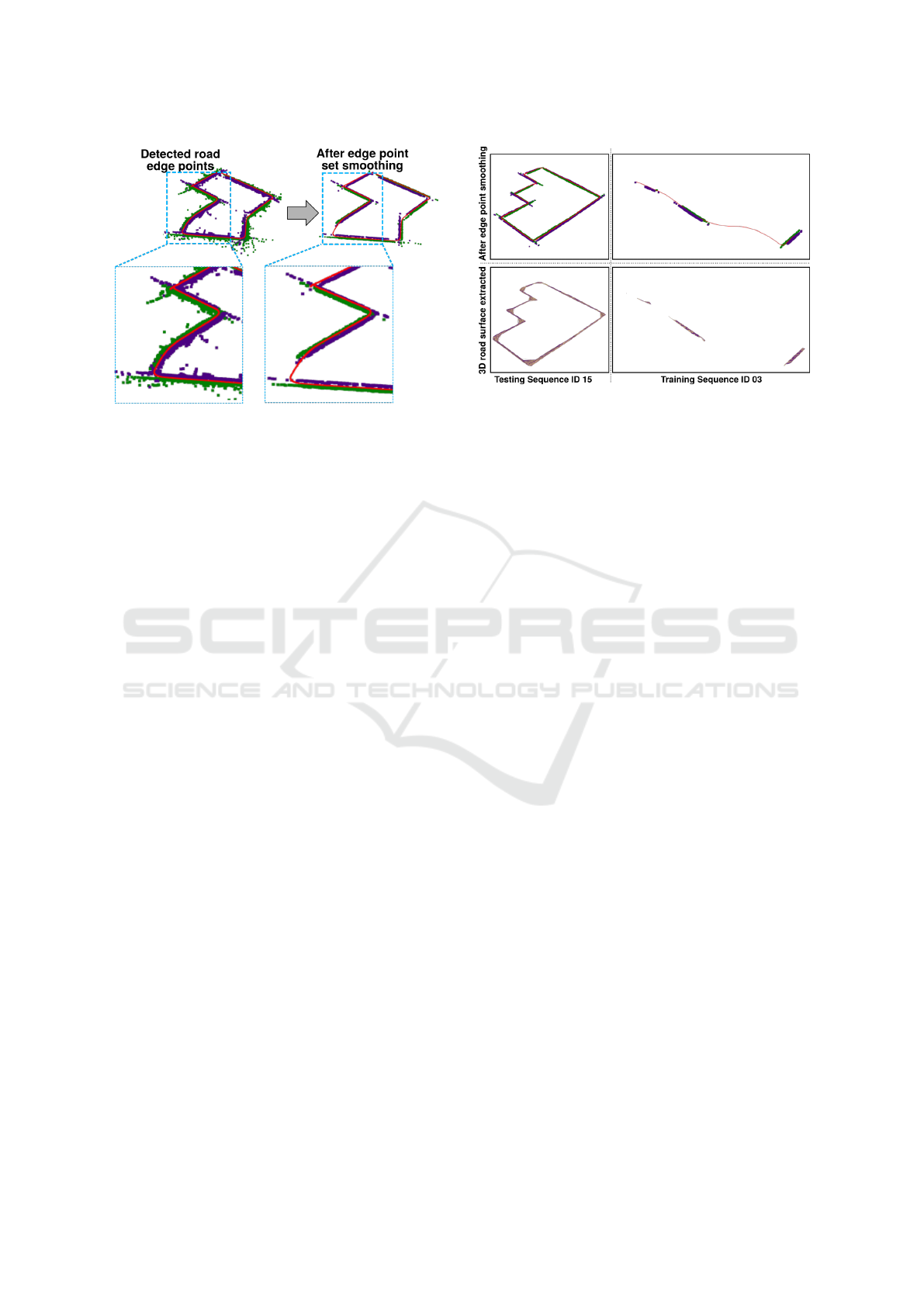
Figure 4: Edge point set smoothing results on sequence 07
data trajectory (top row) with zoomed-in region inset (bot-
tom row). Red, purple and green points show the trajectory,
left and right edge points, respectively.
tracted using detected ground points and “road” (GT)
points are overlaid for demonstrating their similar-
ity. It can be seen that short segments of turning or
connections between straight road segments have also
been effectively covered in the triangulated meshes.
RoSELS has also been entirely implemented on
test sequence 15. As the GT for the test sequences is
not available, we qualitatively compare our extracted
road surface with the reference trajectory using sur-
face and point rendering (Figure 5(Left)). In all se-
quences, including 15, we observe that the road sur-
face mesh preserves the trajectory as its medial skele-
ton (Tagliasacchi et al., 2016), as expected.
However, RoSELS fails to extract the road surface
for the entire trajectory where: (a) the segments with
straight roads are highly fragmented, and (b) the sub-
sequences have comparable segments of curved and
straight roads. When edge points are not identified
for large segments of the road, as seen in training
sequence 03 (Figure 5(Right)), RoSELS extracts the
road surface partially. Surface extraction for a com-
plete trajectory for such scenarios requires an in-depth
study of curved roads, which is beyond the scope of
our current work.
5 CONCLUSIONS
We have proposed and implemented RoSELS, a novel
system for automating 3D road surface extraction for
a sequence of 3D automotive LiDAR point clouds. It
implements a five-step workflow. Firstly, with out-
lier removal and multiscale feature extraction, super-
vised learning using RFC is used for ground point de-
tection. Secondly, the height differences in ground
Figure 5: Results of RoSELS on (Left) a sample sequence
from the test set of SemanticKITTI (Behley et al., 2019),
for which annotations for semantic segmentation have not
been published; and (Right) a sample sequence where the
surface is only partially extracted.
points are used to detect road edge points using the
EM algorithm. Simultaneously, our frame classifica-
tion provides the road geometry by transfer learning
using ResNet-50 on top-view images. The fourth step
is for smoothing the edge point set in the sequence.
As the last step, the 3D road surface is extracted as
a triangulated mesh using 3D Delaunay tetrahedral-
ization. Our experiments on four sequences in Se-
manticKITTI with varying complexity in geometry
have yielded good results, which have been quali-
tatively and quantitatively verified. Thus, RoSELS
works successfully on trajectories with contiguous
straight roads, predominantly.
Although road surfaces across different trajecto-
ries are extracted with a high level of visual similarity
using the proposed algorithm, our approach fails to
extract road surfaces for the entire trajectory where
the segments do not have contiguous straight road ge-
ometry. Thus, extending our method to curved roads
is in the scope of future work. A more robust met-
ric and ground truth for validation are also open chal-
lenges for the road surface extraction application.
ACKNOWLEDGEMENT
We are grateful to Machine Intelligence and Robotics
(MINRO) grant from the Government of Karnataka
for supporting our work through graduate fellowship
and conference support, and to Mayank Sati and Sunil
Karunakaran, who are with the Ignitarium Technol-
ogy Solutions, Pvt. Ltd., for their insightful discus-
sion and suggestions. We thank IIITB and the re-
search group at GVCL for their constant support.
RoSELS: Road Surface Extraction for 3D Automotive LiDAR Point Cloud Sequence
65

REFERENCES
Arora, M., Wiesmann, L., Chen, X., and Stachniss, C.
(2021). Mapping the Static Parts of Dynamic Scenes
from 3D LiDAR Point Clouds Exploiting Ground
Segmentation. In 2021 European Conference on Mo-
bile Robots (ECMR), pages 1–6. IEEE.
Behley, J., Garbade, M., Milioto, A., Quenzel, J., Behnke,
S., Gall, J., and Stachniss, C. (2021). Towards 3d
lidar-based semantic scene understanding of 3d point
cloud sequences: The semantickitti dataset. The Inter-
national Journal of Robotics Research, 40(8-9):959–
967.
Behley, J., Garbade, M., Milioto, A., Quenzel, J., Behnke,
S., Stachniss, C., and Gall, J. (2019). SemanticKITTI:
A dataset for semantic scene understanding of LiDAR
sequences. In Proceedings of the IEEE/CVF Interna-
tional Conference on Computer Vision, pages 9297–
9307.
Besl Paul, J. and McKay, N. D. (1992). A method for regis-
tration of 3-D shapes. IEEE Transactions on Pattern
Analysis and Machine Intelligence, 14(2):239–256.
Breiman, L. (2001). Random forests. Machine learning,
45(1):5–32.
Buitinck, L., Louppe, G., Blondel, M., Pedregosa, F.,
Mueller, A., Grisel, O., Niculae, V., Prettenhofer, P.,
Gramfort, A., Grobler, J., Layton, R., VanderPlas, J.,
Joly, A., Holt, B., and Varoquaux, G. (2013). API de-
sign for machine learning software: experiences from
the scikit-learn project. In ECML PKDD Workshop:
Languages for Data Mining and Machine Learning,
pages 108–122.
Chen, X., Vizzo, I., L
¨
abe, T., Behley, J., and Stach-
niss, C. (2021). Range image-based LiDAR local-
ization for autonomous vehicles. In 2021 IEEE In-
ternational Conference on Robotics and Automation
(ICRA), pages 5802–5808. IEEE.
Chollet, F. et al. (2015). Keras. https://keras.io.
Cortinhal, T., Tzelepi, G., and Aksoy, E. (2021). Sal-
saNext: Fast, Uncertainty-aware Semantic Segmen-
tation of LiDAR Point Clouds for Autonomous Driv-
ing. In 15th International Symposium, ISVC 2020, San
Diego, CA, USA, October 5–7, 2020, volume 12510.
Springer.
Dempster, A. P., Laird, N. M., and Rubin, D. B. (1977).
Maximum likelihood from incomplete data via the
EM algorithm. Journal of the Royal Statistical So-
ciety: Series B (Methodological), 39(1):1–22.
Fischler, M. A. and Bolles, R. C. (1981). Random sample
consensus: A paradigm for model fitting with appli-
cations to image analysis and automated cartography.
Communications of the ACM, 24(6):381–395.
Gigli, L., Kiran, B. R., Paul, T., Serna, A., Vemuri, N., Mar-
cotegui, B., and Velasco-Forero, S. (2020). Road Seg-
mentation on low resolution LIDAR point clouds for
autonomous vehicles. In XXIV International Society
for Photogrammetry and Remote Sensing Congress,
Nice, France. ISPRS 2020.
Guo, Y., Wang, H., Hu, Q., Liu, H., Liu, L., and Ben-
namoun, M. (2020). Deep learning for 3d point
clouds: A survey. IEEE transactions on pattern anal-
ysis and machine intelligence.
He, K., Zhang, X., Ren, S., and Sun, J. (2016). Deep resid-
ual learning for image recognition. In Proceedings of
the IEEE conference on computer vision and pattern
recognition, pages 770–778.
Hu, Q., Yang, B., Xie, L., Rosa, S., Guo, Y., Wang, Z.,
Trigoni, N., and Markham, A. (2020). Randla-net:
Efficient semantic segmentation of large-scale point
clouds. In Proceedings of the IEEE/CVF Conference
on Computer Vision and Pattern Recognition, pages
11108–11117.
Krizhevsky, A., Sutskever, I., and Hinton, G. E. (2012). Im-
agenet classification with deep convolutional neural
networks. Advances in neural information processing
systems, 25.
Kumari, B. and Sreevalsan-Nair, J. (2015). An interactive
visual analytic tool for semantic classification of 3D
urban LiDAR point cloud. In Proceedings of the 23rd
SIGSPATIAL International Conference on Advances
in Geographic Information Systems, pages 1–4.
Liu, Z., Liu, D., Chen, T., and Wei, C. (2013). Curb detec-
tion using 2D range data in a campus environment. In
2013 Seventh International Conference on Image and
Graphics, pages 291–296. IEEE.
Milioto, A., Vizzo, I., Behley, J., and Stachniss, C. (2019).
Rangenet++: Fast and accurate lidar semantic seg-
mentation. In 2019 IEEE/RSJ International Confer-
ence on Intelligent Robots and Systems (IROS), pages
4213–4220. IEEE.
Ouyang, Z., Dong, X., Cui, J., Niu, J., and Guizani, M.
(2021). PV-EncoNet: Fast Object Detection Based on
Colored Point Cloud. IEEE Transactions on Intelli-
gent Transportation Systems, Early Access:1–12.
Paigwar, A., Erkent,
¨
O., Sierra-Gonzalez, D., and Laugier,
C. (2020). Gndnet: Fast ground plane estimation and
point cloud segmentation for autonomous vehicles. In
2020 IEEE/RSJ International Conference on Intelli-
gent Robots and Systems (IROS), pages 2150–2156.
IEEE.
Rist, C. B., Schmidt, D., Enzweiler, M., and Gavrila, D. M.
(2020). SCSSnet: Learning Spatially-Conditioned
Scene Segmentation on LiDAR Point Clouds. In
2020 IEEE Intelligent Vehicles Symposium (IV), pages
1086–1093. IEEE.
Scott, G. J., England, M. R., Starms, W. A., Marcum, R. A.,
and Davis, C. H. (2017). Training deep convolutional
neural networks for land–cover classification of high-
resolution imagery. IEEE Geoscience and Remote
Sensing Letters, 14(4):549–553.
Shen, Z., Liang, H., Lin, L., Wang, Z., Huang, W., and Yu,
J. (2021). Fast Ground Segmentation for 3D LiDAR
Point Cloud Based on Jump-Convolution-Process. Re-
mote Sensing, 13(16):3239.
Shewchuk, J. R. (2002). Constrained Delaunay Tetrahe-
dralizations and Provably Good Boundary Recovery.
In Eleventh International Meshing Roundtable (IMR),
pages 193–204.
Stainvas, I. and Buda, Y. (2014). Performance evaluation
DeLTA 2022 - 3rd International Conference on Deep Learning Theory and Applications
66

for curb detection problem. In 2014 IEEE Intelligent
Vehicles Symposium Proceedings, pages 25–30. IEEE.
Sui, L., Zhu, J., Zhong, M., Wang, X., and Kang, J. (2021).
Extraction of road boundary from MLS data using
laser scanner ground trajectory. Open Geosciences,
13(1):690–704.
Sullivan, C. B. and Kaszynski, A. (2019). PyVista: 3D plot-
ting and mesh analysis through a streamlined interface
for the Visualization Toolkit (VTK). Journal of Open
Source Software, 4(37):1450.
Tagliasacchi, A., Delame, T., Spagnuolo, M., Amenta, N.,
and Telea, A. (2016). 3D Skeletons: A State-of-the-
Art Report. In Computer Graphics Forum, volume 35,
pages 573–597. Wiley Online Library.
Weinmann, M., Jutzi, B., and Mallet, C. (2014). Seman-
tic 3D scene interpretation: A framework combin-
ing optimal neighborhood size selection with rele-
vant features. ISPRS Annals of the Photogramme-
try, Remote Sensing and Spatial Information Sciences,
2(3):181. doi : https://doi.org/10.5194/isprsannals-II-
3-181-2014.
Zhao, L., Yan, L., and Meng, X. (2021). The Extraction
of Street Curbs from Mobile Laser Scanning Data in
Urban Areas. Remote Sensing, 13(12):2407.
Zhou, Q.-Y., Park, J., and Koltun, V. (2018a). Open3D:
A modern library for 3D data processing.
arXiv:1801.09847.
Zhou, Z., Zheng, Y., Ye, H., Pu, J., and Sun, G. (2018b).
Satellite image scene classification via ConvNet with
context aggregation. In Pacific Rim Conference on
Multimedia, pages 329–339. Springer.
Ziou, D. and Tabbone, S. (1998). Edge Detection Tech-
niques - an Overview. Pattern Recognition and Image
Analysis (Advances in Mathematical Theory and Ap-
plications), 8(4):537–559.
RoSELS: Road Surface Extraction for 3D Automotive LiDAR Point Cloud Sequence
67
