A Fault Management Preventive Maintenance Approach in Mobile

Networks using Sequential Pattern Mining

Márcio Pereira

1,3 a

, David Duarte

and Pedro Vieira

2,3 c

CELFINET, Consultoria em Telecomunicações, Lda., Lisboa, Portugal

Instituto Superior de Engenharia de Lisboa (ISEL), Lisboa, Portugal

Instituto de Telecomunicações (IT), Lisboa, Portugal

Keywords: Fault Management, Machine Learning, Preventive Maintenance, Sequential Pattern Mining.

Abstract: Mobile networks' fault management can take advantage of Machine Learning (ML) algorithms making its

maintenance more proactive and preventive. Currently, Network Operations Centers (NOCs) still operate in

reactive mode, where the troubleshoot is only performed after the problem identification. The network

evolution to a preventive maintenance enables the problem prevention or quick resolution, leading to a greater

network and services availability, a better operational efficiency and, above all, ensures customer satisfaction.

In this paper, different algorithms for Sequential Pattern Mining (SPM) and Association Rule Learning (ARL)

are explored, to identify alarm patterns in a live Long Term Evolution (LTE) network, using Fault

Management (FM) data. A comparative performance analysis between all the algorithms was carried out,

having observed, in the best case scenario, a decrease of 3.31% in the total number of alarms and 70.45% in

the number of alarms of a certain type. There was also a considerable reduction in the number of alarms per

network node in a considered area, having identified 39 nodes that no longer had any unresolved alarm.

These results demonstrate that the recognition of sequential alarm patterns allows taking the first steps in the

direction of preventive maintenance in mobile networks.

1 INTRODUCTION

Fault Management (FM) optimization in mobile

networks involves taking advantage of Machine

Learning (ML) techniques to make its maintenance

proactive and preventive.

Mobile network operations still work in reactive

mode, i.e., the diagnosis and the problem solving

starts only after a network malfunction occurs, a

service is impacted, or when a customer complains.

The engineers have access to a lot of information such

as alarms, performance measurements and more, but

they lack an effective way to quickly solve issues.

Thus, Mean Time To Repair (MTTR) is affected,

impacting network and service availability,

operational efficiency, and customer satisfaction.

Minding a solution for preventive maintenance,

operators can leverage ML to reduce operational

costs, improve network and service availability,

https://orcid.org/0000-0003-3354-973X

https://orcid.org/0000-0002-9774-4115

https://orcid.org/0000-0003-0279-8741

improve customer satisfaction, and reduce missed

Service Level Agreements (SLAs). In this context,

the main goal of this paper is to create a solution for

preventive maintenance of mobile networks' alarms,

using real data, that:

1. Mines alarms clusters and establishes

relationships between them, forming

association rules;

2. Continuously learns from new data, improves

over time, and builds expertise in the network

maintenance domain;

3. Defines antecedent and consequent alarms in

a sequential pattern, where they are sorted

chronologically;

4. Recognizes the most frequent patterns in order

to find the most concerning faults and identify

the main advantages that come from their

prevention.

Pereira, M., Duarte, D. and Vieira, P.

A Fault Management Preventive Maintenance Approach in Mobile Networks using Sequential Pattern Mining.

DOI: 10.5220/0011308100003286

In Proceedings of the 19th International Conference on Wireless Networks and Mobile Systems (WINSYS 2022), pages 76-83

ISBN: 978-989-758-592-0; ISSN: 2184-948X

Some recent related work will be presented in the

following. In (Araújo, 2019), the alarms’ proactive

management is addressed as a way to take advantage

of ML algorithms to follow the evolution of mobile

networks and services operations. In (Mulvey, 2019)

and (Nouioua, 2021), research is carried out on the

application of ML techniques and data mining in the

fault management of telecommunications networks,

from an operational point of view. The authors

surveyed several machine learning based techniques

for fault management, including the ones used in this

work.

The paper is organized as follows: Section 2

briefly presents the study carried out on Association

Rule Learning (ARL) and Sequential Pattern Mining

(SPM) algorithms, its methodology and their

respective evaluation metrics. Section 3 presents the

experimental results of all the discussed algorithms'

implementation, with a comparison of their

efficiencies, and finally Section 4 concludes the

paper.

2 METHODOLOGY

2.1 Fault Management Data

The used dataset contains several alarm logs from a

live LTE network. These logs contain the timestamp,

severity, name, type, technology, detailed

information, and the network node associated with

each alarm.

As described in (Huawei, 2015), the alarms can be

classified, as to their severity, as follows:

1. Critical: A critical alarm affects system services.

As soon as it is triggered, immediate actions must

be taken, even when the fault occurs outside

working hours;

2. Major: A major alarm affects the quality of

service and requires immediate action, only if

occurs during working hours;

3. Minor: A minor alarm usually does not affect the

quality of service. It should be treated as soon as

possible or monitored to avoid potential severe

failures;

4. Warning: A warning alarm indicates a possible

error that could affect the quality of service.

Requires different actions depending on specific

errors.

In the sequence, alarms are further categorized by

their type, depending on their operational area:

Power; Environment; Signaling; Trunk; Hardware;

Software; System; Communication; Service quality;

Unexpected operation; Operations and Maintenance

Center (OMC); Integrity; Operation; Physical

resource; Security; Time domain; Running;

Processing.

2.2 Association Rule Learning

Association Rule Learning (ARL) allows extracting

correlations or strong associations, hidden between

sets of items present in transactions in a certain

dataset. The association rules problem defines a

transaction as a set of items where each item can have

different attributes. The used dataset contains several

transactions. An association rule is an implication,

written as 𝐴→𝐶, where A and C are sets of items

called antecedent and consequent, respectively.

Generally, there are two metrics for evaluating an

association rule, support and confidence, presented in

equations (1) and (2), respectively. As datasets

usually store large amounts of information but only

the most frequent transactions are interesting,

minimum values are defined for these evaluation

metrics, which help to filter out less frequent rules.

 Support: Relative frequency or occurrence

probability of a transaction. It can take values

between 0 and 1.

Support(AC) =

Occurrences of A⋃C

l n

f tr

sac

(1)

 Confidence: Probability of a transaction

containing the consequent, knowing that it also

contains the antecedent. Confidence is

maximum if the consequent and the antecedent

always occur together. It is not symmetric, i.e.,

the confidence of AC is different from the

confidence of CA.

Confidence(AC) =

Support(AC)

Support(A)

(2)

In addition to these two metrics, others can be

used to better classify the association rules,

considering other properties that both support and

confidence cannot quantify. In the scope of this work,

three more evaluation metrics were used: lift,

leverage and conviction, and set in equations (3), (4)

and (5), respectively. These metrics were not used to

filter rules, but to better evaluate them.

 Lift: Quantifies how frequent the simultaneous

occurrence of A and C is compared to what

A Fault Management Preventive Maintenance Approach in Mobile Networks using Sequential Pattern Mining

would be expected if they were statistically

independent. If A and C are independent, the

lift will be equal to 1.

Lift(AC) =

Confidence(AC)

Support(C)

(3)

 Leverage: Difference between the frequency

of A and C occurring together and the

frequency that would be expected if A and C

were independent. A value of 0 indicates

independence between the two itemsets.

Leverage(AC) = Support(A

C) – Support(A) × Support(C)

(4)

 Conviction: A high value means that C is

strongly dependent on A. For example, if the

confidence is equal to 1, the denominator will

be 0, so the conviction will be

∞. Like lift, if

the items are independent, the conviction is

equal to 1.

Conviction(AC) =

  ()

 ()

(5)

Under this work, three ARL algorithms were

implemented: Apriori, Equivalence CLAss

Transformation (ECLAT) and Frequent Pattern

(FP)Growth, and extracted from (Agrawal, 1994),

(Zaki, 2000) and (Han, 2004), respectively.

2.2.1 Apriori

This algorithm has to access the dataset several times

to obtain the frequent itemsets. In the first access, the

support is counted for each item individually (level 1

itemsets). Then, with a minimum defined support

value, S, there are excluded rare items, i.e., those

whose support is lower than S.

In later accesses, higher-level itemsets containing

rare items are no longer considered, because if an

item’s support, S

, is lower than S, then all subsets that

contain it will have a support equal or lower than S

and, thus, lower than S (Apriori property).

This process is repeated until there are no more

frequent itemsets to evaluate. The final list of frequent

items is the junction of all the lists created for each

level, including the support values calculated for each

frequent itemset.

2.2.2 ECLAT

ECLAT is an improved version of the Apriori

algorithm. While Apriori uses a horizontal dataset

representation, ECLAT transforms it into its vertical

representation where, instead of indicating the

itemsets that belong to each transaction, it lists the

transactions in which item occurs.

Transaction lists for higher level itemsets are

created recursively, calculating the intersection of the

transaction lists (from the previous level) of each

item. If the intersection is null, the itemset is removed

from the list. This process is over when, for a certain

level, all intersections are null.

If the minimum support is set to the same value,

the final list of frequent itemsets will be identical to

that of the Apriori algorithm. However, ECLAT takes

up less memory throughout its process, manages to be

faster by using a vertical approach – in which its

calculations are done in parallel – and ends up

performing fewer accesses to the dataset, because it is

possible to calculate the support values for any level.

2.2.3 FPGrowth

The FPGrowth algorithm implementation considers

the Frequent Pattern (FP)-tree, a tree that contains the

prefixes of the transactions. Each tree path represents

a set of transactions that share the same prefix, where

each node corresponds to a single item. Furthermore,

all nodes referring to the same item are linked

together, so that all transactions that contain a certain

item can be easily found and accounted for when

traversing this tree.

The main operation that the FPGrowth algorithm

has to perform is to build the FP-tree of a projected

dataset, i.e., a dataset with the transactions that

contain a certain item, with that item removed. This

projected dataset is processed recursively, not

forgetting that the frequent itemsets found share the

same prefix – the item that was removed.

After building the FP-trees for all the necessary

dataset projections, the process of eliminating some

of the nodes associated with rare items is carried out

in order to simplify the tree and speed up the process.

Thanks to an efficient implementation of FP-trees,

the FPGrowth algorithm largely outperforms the

previously presented algorithms (Apriori and

ECLAT), both in terms of execution time and the

memory required, since the storage of the dataset

using a tree representation is more compact than the

full list of transactions.

2.3 Sequential Pattern Mining

Sequential Pattern Mining (SPM), unlike ARL, takes

into consideration the items’ order in each sequence,

allowing to discover frequent patterns in a dataset,

which may prove useful or interesting to be explored.

WINSYS 2022 - 19th International Conference on Wireless Networks and Mobile Systems

The objective of SPM algorithms is to find all

patterns (sub-sequences) that have a support higher

than or equal to the minimum support value defined

by the user. Therefore, the patterns they each find are

the same for all the algorithms. What differentiates

them is solely their efficiency in recognizing those

patterns.

Three SPM algorithms were also implemented:

PrefixSpan, Sequential PAttern Discovery using

Equivalence classes (SPADE) and Sequential

PAttern Mining (SPAM), and extracted from (Pei,

2004), (Zaki, 2001) and (Ayres, 2002), respectively.

2.3.1 PrefixSpan

PrefixSpan is a pattern-growth algorithm, based on

FPGrowth. It is the only one of the three studied

algorithms that does not consider all possible

combinations for the patterns that can be found.

Recursively accesses the dataset to concatenate new

items until the complete pattern is formed, therefore,

it only considers the patterns that exist in the dataset.

These successive accesses can, however, be time

consuming, so the concept of “projected dataset” was

introduced, to reduce its size, optimizing the access.

In terms of memory, creating multiple dataset

projections can take up a lot of data storage space.

2.3.2 SPADE

Inspired by ECLAT, this algorithm uses a vertical

representation of the dataset, created during the first

access, indicating in which itemsets and in which

sequence each of the items is found.

The vertical representation has two interesting

properties for recognizing sequential patterns. The

first property is that the list created for any sequence

allows directly calculating its support. The second

property is that the list of any sequence can be

obtained, without directly accessing the original

dataset, by joining the various lists of the sub-

sequences that compose it.

By taking advantage of these properties,

algorithms such as SPADE and even SPAM perform

their discovery for sequential patterns without

repeatedly accessing the dataset and, therefore,

without keeping many patterns in memory.

2.3.3 SPAM

Similar to the algorithm presented above, SPAM

manages to be even more efficient by optimizing the

structure of the pattern list. This algorithm encodes

these lists as binary vectors, which cuts the memory

necessary to store the same information. In addition,

it speeds up the mathematical operations that need to

be performed. It can still be improved with the use of

compression techniques that reduce the number of

used bits.

This algorithm has been shown to be faster than

SPADE and PrefixSpan, especially for relatively

large datasets. In terms of memory, SPADE still

manages to be the more efficient of the two.

3 EXPERIMENTAL RESULTS

In order to discover the association rules and

sequential patterns within the network, real FM data

were used to test, analyse, and compare the presented

algorithms.

To evaluate every association rule, the minimum

support value was set to “2 occurrences / Total

number of transactions”, i.e., it only takes a repetition

for an itemset to be considered frequent. A minimum

confidence of 50% was also imposed, which indicates

that, at least half of the transactions that contain the

antecedent also contain the consequent (group of

alarms).

Before analysing the results and to assess the

efficiency of each algorithm, the execution times and

the used memory were quantified. These results were

obtained from tests performed on a machine with the

following specifications: Intel® Core™ i5-7300HQ

CPU @ 2.50GHz (4 CPUs), 8GB RAM, Windows 10

Education 64bits.

3.1 Association Rule Learning

In the implementation of the algorithms Apriori and

FPGrowth, the MLxtend library (Raschka, 2018) was

used. For ECLAT, it was used the PyFIM library

(Borgelt, 2012). The tests were carried out for a time

window from 1 to 30 minutes, and with one minute

granularity. Comparative graphs for the different time

windows are shown in Figure 1 and Figure 2, for the

execution time and memory usage, respectively.

Figure 1: Execution time of each ARL algorithm, for

several time windows.

A Fault Management Preventive Maintenance Approach in Mobile Networks using Sequential Pattern Mining

As in Figure 1, the execution time of all

algorithms decreases as the time window increases.

Although, with this growth, there are transactions

with more sets of items, the number of transactions

decreases and, also, there are fewer evaluation

metrics to calculate, which can justify the time

reduction. Comparing the executions time of each

algorithm, it is possible to verify that the fastest is

FPGrowth, followed by ECLAT and, finally, Apriori.

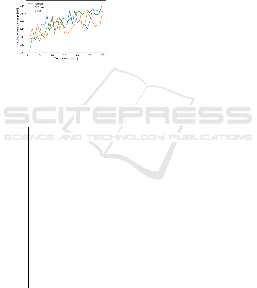
Figure 2: Memory usage of each ARL algorithm, for several

time windows.

Considering Figure 2, despite constant

fluctuations, it is possible to verify that the used

memory increases as the time window increases,

which is justified by the growth of the number of

items in each transaction. In general, it is possible to

conclude that the most efficient in terms of memory

occupation is also FPGrowth. ECLAT manages to be

very optimized for small transactions, but after a

certain point, it uses even more memory than Apriori.

The list of rules, identical to all algorithms, was

sorted by the Lift metric in descendent order, since

those with the higher value are the ones with a greater

dependence between the rule’s antecedent and

consequent. The top 6 rules are shown in Table 1. The

confidence and conviction metrics were omitted as

they were the same for all evaluated relations and

time windows, having the values 1 and ∞ ,

respectively.

Despite the support values being low, the

algorithms demonstrate conviction that these

associations are quite strong, i.e., when a certain

antecedent alarm occurs, the consequent alarm will

occur in the following.

Note that, for a given time window and network

node, there is always a pair of symmetric rules, i.e.,

there is always a second rule where the antecedent is

the consequent, and the consequent is the antecedent

of the first rule. Therefore, at this stage, it is not

possible to be sure about the order of occurrence of

the alarms, and it is necessary to move forward

resorting to Sequential Pattern Mining (SPM).

Table 1: The top 6 association rules, and respective evaluation metrics calculated by the three algorithms, with greater Lift.

Minute(s) Network node Antecedent(s) Consequent(s) Support Lift Leverage

–

BX94BL

RF Unit ALD

Current Out of Range

ALD Maintenance Link

Failure

0.00134

–

0.00157

741.5

–

634.0

0.00134

–

0.00157

–

BX94BL

ALD Maintenance

Link Failure

RF Unit ALD Current Out of

Range

0.00134

–

0.00157

741.5

–

634.0

0.00134

–

0.00157

–

VA08OL X2 Interface Fault

Inter-System Cabinet

Configuration Conflict

0.00151

–

0.00158

662.0

–

632.0

0.00150

–

0.00157

–

VA08OL

Inter-System Cabinet

Configuration

Conflict

X2 Interface Fault

0.00151

–

0.00158

662.0

–

632.0

0.00150

–

0.00157

2 BX16QL Certificate Invalid

External Clock Reference

Problem

0.00202 494.0 0.00202

2 BX16QL

External Clock

Reference Problem

Certificate Invalid 0.00202 494.0 0.00202

WINSYS 2022 - 19th International Conference on Wireless Networks and Mobile Systems

3.2 Sequential Pattern Mining

In the implementation of the algorithms, the extensive

framework for data mining SPMF (Fournier-Viger,

2016) was used.

In the previous section, it was noticed that there

was no need to test several time windows (1 to 30

minutes, every minute) in the definition of

transactions, as the results were similar for all of

them. Therefore, for these algorithms, transactions

were defined based on a single dynamic window.

Additionally, there is a timeout interval in which if no

alarm happens during that interval, the next alarm that

occurs will belong to the next transaction.

The timeout value was defined considering the

predominant association rules in the previous section,

namely those that contained alarms associated with

the Antenna Line Device (ALD). Since the objective

is to have this pair of alarms always in the same

transaction, the timeout was fixed at 11 minutes,

because this is the maximum time interval registered

between the two alarms.

The execution times and memory usage of each

algorithm were measured, for the dynamic window,

and are presented in Table 2.

Observing the average value of three tests

executed in a row, the fastest algorithm is the SPAM,

followed by PrefixSpan, and finally SPADE. In terms

of used memory, the order is reversed, with SPADE

being the most efficient, followed by PrefixSpan and,

finally, SPAM.

Table 2: Execution times and memory usages of each

algorithm, for the dynamic time window.

Algorithm Execution time

Maximum

memory

usage

PrefixSpan 14 minutes 43 seconds 179.07 MB

SPADE 15 minutes 9 seconds 178.06 MB

SPAM 13 minutes 50 seconds 180.18 MB

The list of patterns, identical to all algorithms,

was sorted by the Lift metric in descendent order, as

those with this highest value are those with a greater

dependency among all the alarms that make up the

pattern. The top 5 patterns are shown in Table 3.

As already noticed, the same alarms that had

already appeared in the association rules of the

previous section continue to be present. However, in

this analysis, there are no longer symmetrical rules,

only the patterns, which, by themselves, already

indicate the real order in which the alarms occur.

All listed patterns have been analysed using the

alarm’s vendor documentation. Furthermore,

assuming that when the antecedent is solved, the

consequent no longer happens, and that the time

interval between them is sufficient to report and solve

the failure, the consequent will be removed from the

original dataset, and the maximum reduction in the

number of alarms will be calculated.

The next sections will present some use cases

considering the patterns found in Table 3.

Table 3: The top 5 sequential patterns, and respective evaluation metrics calculated for the three algorithms, with greater Lift.

Network node Pattern Support Confidence Lift Leverage Conviction

VA08OL

{Inter-System Cabinet

Configuration Conflict, X2

Interface Fault}

0.00259 1.0 386.5 0.00258

∞

VA83WL

{RF Unit ALD Current Out of

Range, ALD Maintenance Link

Failure}

0.00274 1.0 364.33 0.00274 ∞

BX16QL

{Certificate Invalid, External Clock

Reference Problem}

0.00197 0.66 226.0 0.00196 2.9912

AB42AL

{Inter-System Cabinet

Configuration Conflict, X2

Interface Fault}

0.00476 1.0 210.0 0.00474 ∞

TX49BL

{ALD Maintenance Link Failure,

External Clock Reference Problem}

0.00477 1.0 209.66 0.00475

∞

A Fault Management Preventive Maintenance Approach in Mobile Networks using Sequential Pattern Mining

3.2.1 RF Unit ALD Current out of Range 

ALD Maintenance Link Failure

In the context of preventive maintenance, it is

necessary to understand the benefits of being able to

recognize the patterns that happened in the past, in

order to predict and prevent what will happen in the

future. In this case, by preventing the antecedent

alarm, RF Unit ALD Current Out of Range, 715

“ALD Maintenance Link Failure” alarms are avoided.

This mainly translates into the reduction of the

number of alarms as follows:

 “Communication” type alarms: 1860  1145

(-38.44%);

 “VX73KL” node alarms: 40  22 (-45%);

 “CS12KL” node alarms: 87  51 (-41.38%);

 “VX37KL” node alarms: 179  107 (-

40.22%);

 “CR29VL” node alarms: 64  44 (-31.25%).

3.2.2 Inter-System Cabinet Configuration

Conflict  X2 Interface Fault

By solving the errors and configuration conflicts in

the cabinet, 6327 “X2 Interface Fault” alarms can be

prevented from happening. This means a reduction

of:

 Total number of alarms: 191053  184726 (-

3.31%);

 “Signaling” type alarms: 8981  2654 (-

70.45%);

 “LO01AL” node alarms: 37  18 (-51.35%);

 “VX83EL” node alarms: 74  37 (-50%);

 “VX49KL” node alarms: 53  27 (-49.06%).

3.2.3 Certificate Invalid  External Clock

Reference Problem

By properly validating the certificate, it can prevent a

lot of “External Clock Reference Problem” alarms

from happening. As this pattern shares the same

consequent as the next, the calculation and analysis of

this impact is made for the next pattern.

These two patterns are between “Major” alarms,

while the first two were between a “Minor”

antecedent and a “Major” consequent. This allows to

deduce, after analysing the 4 cases, that the sequence

of alarms always follows an increasing order in terms

of severity. Of course, there are alarms caused by

other ones with the same severity, but a less severe

alarm than the previous one is unlikely to occur (for

example, Major → Minor).

3.2.4 ALD Maintenance Link Failure 

External Clock Reference Problem

This pattern is the second (from the ones presented)

in which the “External Clock Reference Problem”

alarm is found as a consequence. This suggests that

the problems in the external clock reference can be

indirectly caused by various sources on the network,

which leads to a bad configuration of the clock or the

malfunction of some hardware element, essential for

proper clock synchronization.

Resuming the correct external reference clock

synchronization, it prevents the occurrence of 1414

“External Clock Reference Problem” alarms. This

mainly translates into the reduction of:

 “Hardware” type alarms: 7969  6555 (-

17.74%);

 There are 39 nodes that no longer have any

unresolved alarm (-100%);

 “VX30EG” node alarms: 18  1 (-94.44%);

 “CR06VU” node alarms: 22  4 (-81.82%);

 “VX88EU” node alarms: 50  12 (-76%).

Hence, it is concluded that, with sequential

pattern mining, it is possible to predict which will be

the most likely alarm to be the consequence of a given

antecedent alarm. Within the scope of preventive

maintenance, if the problem resolution is quick and

effective, it is possible to completely prevent the

consequent alarm from occurring, resulting in a

decrease in the number of triggered alarms and

failures caused by them.

4 CONCLUSIONS

This work aimed to develop and test a solution for

proactive and preventive maintenance in LTE mobile

networks, by using fault management data. Two types

of machine learning techniques for handling this data

were explored: ARL and SPM.

For the ARL algorithms, FPGrowth presented the

best performance in terms of execution time and used

resources. ECLAT was the most efficient for short

transactions, being surpassed by Apriori for larger

transactions. In all of them there was a symmetry in

the association rules, having therefore evolved to the

SPM algorithms, where the order of alarms’

occurrence is strongly important.

For the SPM algorithms, SPAM was the most

efficient in terms of execution time, but the worst in

terms of resource utilization. SPADE was the most

efficient in terms of resource utilization but the

slowest of all. On the other hand, PrefixSpan offered

WINSYS 2022 - 19th International Conference on Wireless Networks and Mobile Systems

a good compromise among all. In all the performed

tests, it was possible to conclude that the prevention

of consequent alarms results in a decrease in their

absolute number in the network’s nodes where they

occurred.

In the best case scenario, there was a decrease of

3.31% in all analysed nodes, and 70.45% in terms of

alarms of the same type. It was also noticed that 39

network nodes no longer had any unresolved alarm.

These results demonstrate that sequential pattern

mining drives the preventive maintenance of alarms

in a LTE mobile network, reinforcing the preventive

maintenance’ importance for Mobile Network

Operators (MNOs).

ACKNOWLEDGEMENTS

This work was carried out in the scope of the

international project Cognitive and Automated

Network Operations for Present and Beyond

(CANOPY) AI2021-061, under the CELTIC-NEXT

Core Group and the EUREKA Clusters program. The

authors would like to thank the COMPETE/FEDER

program for funding the national component of the

project (14/SI/2021), as well as the Instituto de

Telecomunicações (IT) and CELFINET for its

support.

REFERENCES

C. G. Araújo, G. Cardoso, J. Sousa, M. Coutinho, P. Neves

(2019). “Predictive fault management,” in InnovAction

#4, Altice Labs.

D. Mulvey, C. H. Foh, M. A. Imran and R. Tafazolli (2019).

“Cell Fault Management Using Machine Learning

Techniques,” IEEE Access, vol. 7, pp. 124514-124539.

M. Nouioua, P. Fournier-Viger, G. He, F. Nouioua, and M.

Zhou (2021). “A survey of machine learning for

network fault management,” in Machine Learning and

Data Mining for Emerging Trend in Cyber Dynamics.

Huawei (2015). 3900 Series Base Station Product

Documentation, V100R010C10. Huawei Technologies

Co..

R. Agrawal and R. Srikant (1994). “Fast algorithms for

mining association rules in large databases,” in

Proceedings of the 20th International Conference on

Very Large Data Bases, VLDB ’94, (San Francisco,

CA, USA), p. 487–499, Morgan Kaufmann Publishers

Inc..

M. Zaki (2000). “Scalable algorithms for association

mining,” IEEE Transactions on Knowledge and Data

Engineering, vol. 12, 3, pp. 372–390.

J. Han, J. Pei, Y. Yin, and R. Mao (2004). “Mining frequent

patterns without candidate generation: A frequent-

pattern tree approach,” Data Mining and Knowledge

Discovery, vol. 8, pp. 53–87.

J. Pei, J. Han, B. Mortazavi-Asl, J. Wang, H. Pinto, Q.

Chen, U. Dayal, and M. Hsu (2004). “Mining sequential

patterns by pattern-growth: The prefixspan approach,”

IEEE Transactions on Knowledge and Data

Engineering, vol. 16, pp. 1424–1440.

M. Zaki (2001). “SPADE: An efficient algorithm for

mining frequent sequences,” Machine Learning, vol.

42, pp. 31–60.

J. Ayres, J. Flannick, J. Gehrke, and T. Yiu (2002).

“Sequential pattern mining using a bitmap

representation,” in Proceedings of the Eighth ACM

SIGKDD International Conference on Knowledge

Discovery and Data Mining, KDD ’02, (New York,

NY, USA), p. 429–435, Association for Computing

Machinery.

S. Raschka (2018). “MLxtend: Providing machine learning

and data science utilities and extensions to python’s

scientific computing stack,” The Journal of Open

Source Software, vol. 3.

C. Borgelt (2012). “Frequent item set mining,” WIREs Data

Mining and Knowledge Discovery, vol. 2, 6, pp. 437–

456.

P. Fournier-Viger et al. (2016). “The SPMF Open-Source

Data Mining Library Version 2,” in Machine Learning

and Knowledge Discovery in Databases (B. Berendt, B.

Bringmann, É. Fromont, G. Garriga, P. Miettinen, N.

Tatti, and V. Tresp, eds.), (Cham), pp. 36–40, Springer

International Publishing.

A Fault Management Preventive Maintenance Approach in Mobile Networks using Sequential Pattern Mining