
Electric Power System Operation: A Technique to Modelling, Monitoring
and Control via Petri Nets
Milton Bastos de Souza
1 a
, Evangivaldo Almeida Lima
2 b
and J
`
es Jesus Fiais Cerqueira
3 c
1
´
Area Automac¸
˜
ao Industrial, Campos Integrado de Manufatura e Tecnologias Senai-Cimatec, Bahia, Salvador, Brazil
2
Exact Sciences Department, State University of Bahia, Salvador, Brazil
3
Electrical Engineering Department, Polytechnic of Federal University of Bahia, Salvador, Brazil
Keywords:
Petri Nets, Electric Power System, Modelling, Monitoring, Control, Switch Breaker, Disconnect Switch.
Abstract:
Petri nets have been widely used as a tool to model, monitor and control several kind of systems. In this paper,
Petri nets are used to model, monitor and control Electrical Power Systems (EPS). The electric power model
will be expanded through a linear transformation. The restrictions imposed for that expansion specialize the
new places with attributes that allow to monitor or control the dynamics of the original Petri net.
1 INTRODUCTION
Modern systems of production have been presenting
high complexity degrees, modeling, analysis, plan-
ning, monitoring and controlling. These systems of
production require appropriate modeling tools to en-
sure and validate the right procedures for their opera-
tions. The Electric Power Systems (EPS) can be clas-
sified as a class of such systems (Tekiner-Mogulkoc
et al., 2012).
Generally, in the study of an EPS is considered
that its operation should occur predominantly in a
steady state. In this case, all of them the load changes,
the opening or closing of disconnectors, the breakers,
or any other occurrence that can generate transients in
the power system are not considered. Thus, all vari-
ables are manipulated with dependence only on time
in the strictly mathematical sense (Weiss and Schulz,
2015). However, when the dynamics of operation of
an EPS is analyzed [i.e. the analysis through the con-
ditional variables that although have a duration asso-
ciated with their occurrence, they do not have any de-
pendence on time to occur], its operation can be con-
sidered as a system whose dynamic is event-driven
[i.e. it can be manipulated as a Discrete Event System
(DES)] (Amini et al., 2019).
Originally, a dynamic system is considered as a
Discrete Event System (DES) if its dynamic [i.e. its
a
https://orcid.org/8265-2459-2141-3657
b
https://orcid.org/3664-7680-0086-3560
c
https://orcid.org/0000-0003-4072-0101
states] is such that it can be considered as having no
dependence on time, but it can be considered as hav-
ing dependence on occurrences or events that can be,
for instance, random. The elapsed time of the event
is token usually as negligible. Afterward, some appli-
cations have presented dependence on timed occur-
rences or events. To deal with such requirements the-
oretical extensions taking into account timed events
were developed. Several are the tools used to study
DES for different kinds of systems. There exist
also some systems with certain operational features
such that they have dynamic called hybrid systems.
Among the main tools used in the study of DES, one
can point out Finite State Automata, Dioids, Queue
Theory, and Petri Nets (Papadopoulos et al., 2019;
Wu et al., 2019; Komenda et al., 2018; Lin et al.,
2016).
Petri net is a well known DES tools. Its pop-
ularity comes mainly due to two factors: it has a
compact representation and also has a graphic repre-
sentation very easy. Over time, the Petri nets have
been incorporating several resources to become them,
more powerful as for instance Continuous Petri net
and timed Petri net. These things have guaranteed for
them, greater information richness in the applications
and also allowed them can be applied to new classes
of systems as for instance EPS (Murata, 1989; Cas-
sandras and Lafortune, 2009; David and Alla, 1994;
Bin et al., 2015; Fendri and Chaabene, 2019).
The Modelling of a DES is building of model to
represent its dynamic [i.e. the evolution of its states
or events] using some suitable tool. The monitoring
Bastos de Souza, M., Lima, E. and Cerqueira, J.
Electric Power System Operation: A Technique to Modelling, Monitoring and Control via Petri Nets.
DOI: 10.5220/0011312100003271
In Proceedings of the 19th International Conference on Informatics in Control, Automation and Robotics (ICINCO 2022), pages 649-657
ISBN: 978-989-758-585-2; ISSN: 2184-2809
Copyright
c
2022 by SCITEPRESS – Science and Technology Publications, Lda. All rights reserved
649

of a DES is the regular observation and recording of
activities that have been occurring in such a system. It
is a process of routinely collecting information about
all states ([i.e. events] of the system. On the other
hand, the basic idea behind controlling of a DES is to
restrict the behavior of the system according to rules
imposed by a controller. This restriction can be en-
forced by enabling or disabling controllable transi-
tions [i.e. events] under some established conditions
previously. For all of them, the Petri nets have been
being shown as a suitable tool (Giua, 1992; Krogh and
Holloway, 1991; Holloway et al., 1996; Dideban and
Alla, 2009).
The EPS has some dynamic features that are de-
pendent on the occurrences of events. The perfor-
mance of maneuvering and protection devices are in-
stances of elements whose dynamics can be com-
pletely modeled based on events. High levels of
safety, quality, reliability and availability are some re-
quirements in the EPS operation. An important fac-
tor in contributing to the fulfillment of these require-
ments is the existence of some modeling tool that al-
lows an observation step-by-step of the evolution of
an EPS in its varied stages. Traditionally, an EPS has
been worked using contact diagrams and their simu-
lation. This technique is inefficient when the systems
become more complex [i.e. when more sophisticated
interlocks are required)].
This work is complemented with a section about
Petri nets and supervisory control theory In the fol-
lowing subsection is done an introduction about lin-
ear transformation to expand a Petri net after that a
vision of monitoring and control. The third section is
an introduction to EPS and in the fourth section, an
application is used to validate the theory presented in
the preview sections. The Conclusion are presented
the mains results (Souza et al., 2016).
2 PETRI NETS
Petri nets consist of a set of tools with graphic and
mathematics resources that are fitted well to a set of
applications in DES. They were used initially to cre-
ate causal relationships among conditions and events
in computer systems and currently present a power-
ful formalism for the DES. Petri nets can provide the
dynamic behavior of a DES. It is possible to verify,
for instance, whether there is parallelism or conflict
between transitions, whether there is a possibility of
occurrence of some event, as well as to follow the
evolution of the system. The content of the section
can be found especially in (Murata, 1989; David and
Alla, 1994; Cassandras and Lafortune, 2009).
Figure 1: Petri Net Composition.
Graphically, a Petri net consists of a graph with
three types of elements: places, transitions and di-
rected arcs connecting places to transitions or transi-
tions to places. Usually, places are represented by cir-
cles, while transitions are represented by narrow bars.
In Figure 1 is shown an instance of Petri net contain-
ing three places (P
1
, P
2
e P
3
), four transitions (t
1
, t
2
,
t
3
and t
4
) and eight arcs connecting places to transi-
tions or transitions to places. Mathematically, a Petri
net can be defined as a quadruple R = hP, T, Pre, Posti
where P is a finite set of places, T is a finite set of
transitions, Pre is a function that defines arcs link-
ing places to transitions and Post is a function that
defines arcs from transitions to places. The arcs can
be weighted. If an arc Pre(P,t) = k or Post(P,t) = k
then the weight of such arc is k. When k = 1, it
does not need to be written. In Figure 1, the arcs
Pre(P
2
,t
3
) = 3 and Post(P
2
,t
4
) = 3 are weighted by
3 and Pre(P
2
,t
1
) = 1, Pre(P
1
,t
2
) = 1, Pre(P
3
,t
4
) = 1,
Post(P
1
,t
1
) = 1, Post(P
2
,t
2
) = 1 and Post(P
3
,t
3
) = 1
are weighted by 1.
On the other hand, the markup of a Petri net is a
mapping M : P → N that associates an integer number
of marks or token to each place. Consequently, M(p)
indicates the number of marks present in a place P.
A marked Petri net is a double N = hR, M
0
i where
R = hP, T, Pre, Posti and M
0
is the initial marking.
The marks M are information assigned after the
transition firing to represent the state evolution of the
network at a given moment. Thus, to simulate the
dynamic behavior of DES, the marking of a Petri net
is modified after each action performed [i.e. each fired
transition].
The evolution of marks can be made by enabling
and firing transitions. A transition t is enabled if, and
only if, in each of its input places P contains at least
the number of marks equal to the weight of the arc
that is connecting P to t. In Figure 1, all transition t
are enabled.
The enablement is denoted by M[t]. The firing of
a transition t removes from each place P the number
of marks equal to the weight of the arc connecting P
[i.e. Pre(P, t)] to t. Besides, the firing of such tran-
sition will deposit at each outlet place P the number
ICINCO 2022 - 19th International Conference on Informatics in Control, Automation and Robotics
650

of marks equal to the weight of the arc connecting t
to P [i.e. Post(P, t)]. Mathematically, the firing of the
transition t in a M-marking leads to a new marking
M
0
= M − Pre(., T ) + Post(., T ).
Any M-marking achievable from the initial mark-
ing M
0
by firing a sequence σ = t
1
t
2
··· t
n
can be writ-
ten as
M
0
= M
0
+ B(P, t) ∗ σ (1)
where σ : T → N is the count vector and B(P, t) =
Post(P, t)− Pre(P, t) is called Incidence Matrix.
The Incidence Matrix provides the balance of the
marks when the firing of transitions occurs. The set
of all reachable marking from an M-marking in n is
called A(n, M). The behavior of a Petri net can be de-
scribed by a graph of reachability GA(N, M
0
), whose
nodes correspond to the achievable markings. In this
graph, there is a tagged arc from node M[t 7→ M
0
] to
node M
0
.
2.1 Supervisory Control using Petri
Nets
In DES, supervisors or controllers are places added
to a Petri net to avoid the occurrence of undesir-
able or prohibited states in the original model of
a plant(Moody and Antsaklis, 2000). The states
reached by the controller enable which states the plant
can reach. The next subsection will present supervi-
sory control using the place invariant property of Petri
net models.
2.2 Development of Supervisor based
on Place Invariants
Many researchers have been using Petri nets as a tool
to model, analyze and synthesize control laws for
DES (Murata, 1989).
Let be the Petri net model for a plant is (N, M
0
),
where N = (P, T, B,W ) is the graph with all its reach-
able markings. Let be also the control purpose is re-
stricting the evolution of the state of the plant S to
a subset S
0
, where this subset S
0
is described by the
group of linear inequalities
L
1
.
.
.
L
q
∗ M(k) ≤
b
1
.
.
.
b
q
, (2)
or L ∗ M(k) ≤ b, Where L ∈ Z
q×n
, b ∈ Z
n
, and oper-
ator “ ≤
00
must be applied element to element.
The control goal is to prevent the firing of certain
transitions. The controller implementation is done by
inserting new Pc
1
, . . . , Pc
q
and their respective tokens
M
c
(k) ∈ N
q
0
which express the state of the controller.
Both the initial marking and the way the controller
is connected to the transitions of the plant model can
be obtained by considering an extended Petri net with
the marking (M, M
c
). If a transition t
j
is fired, the
state of the extended Petri net is changed according
to the equation.
M(k + 1)
M
c
(k + 1)
=
M(k)
M
c
(k)
+
B
B
c
∗σ
j
, (3)
where σ
j
is the nth firing sequence vector in Z
m
and
B
c
is unknown part of the incidence matrix.
A convention needs to be adopted such that for
any pair Pc
i
and t
j
, i = 1, . . . n, j = 1, . . . m, be taken
a arc of Pc
i
to t
j
or t
j
for Pc
i
. With this, a array B
c
can be defined to specify the structure of connection
between the controller and the plant transitions and
thus to have the incidence matrix B
+
c
as the positive
values of B
c
and B
−
c
as negative values B
c
.
The unknown parameters of the M
c
(0) controller
and B
c
can be determined as following:
1. The Control specifications are given from Equa-
tion(2). So, one can do
L ∗ M(k) + M
c
(k) = b, (4)
where k = 0, 1, . . . m and M
c
(k) is a positive vector
of integers inserted to remove the inequality. The
initial marking is gotten doing k = 0 as
M
c
(0) = b − L ∗ M(0); (5)
2. Multiplying both sides of Equation(3) by the ma-
trix [L I] and then applying invariance prop-
erty from the Equation(4), it is determined that the
controller incidence matrix is given by:
B
c
= −L ∗ B (6)
The Equations(5) and (6) are used for solve super-
visor control problems. The Equation(5) is used to
compute initial marking to the controller. The Equa-
tion(6) show how places controller are connected with
plant transitions (Zhou et al., 1992).
Theorem 1. The control produced by Petri net (N,
M0) and constraints established in the Equation(2)
by Equations(5) and (6) is at least restrictive or min-
imally permissive.
Proof 1. The Equation(4) remains constant ∀k =
0, 1, . . . , m of the closed loop system. Thus, as-
sume that the closed-loop system is in the state
(M
0
(k), M
0
c
(k))
0
, and that the transition t
j
is disabled
is to say that:
M(k)
M
c
(k)
≥
B
−
B
−
c
∗ σ
j
which is a necessary condition for not availability of
the transition from PN. This is possible if:
Electric Power System Operation: A Technique to Modelling, Monitoring and Control via Petri Nets
651

• or M
i
(k) < (B
−
∗ q
j
)
i
for any i ∈ {1, . . . , n}, i.e.
the transition is disabled in the PN uncontrolled
(N,M
0
)
• or for some i ∈ {1, . . . m} M
c
i(k) < (B
−
c
∗ σ
j
)
i
=
L
i
∗ B ∗ σ
i
, e M
c
i(k) = b
i
− L
i
∗ M(k) can be found
that b
i
< L
i
∗ M
c
i(k) + L
i
∗ M(k)
Meaning that the transition t
j
could fire the state
M(k) Petri net open loop (N, M
0
), the resulting
state M(k + 1) = M(k) + B ∗ σ
j
would violate the
specification given in Equation(2). Consequently, it
showed that the transition t
j
is disabled in the state
(M
0
(k), M
0
c
(k))
0
of the closed-loop system if and only
if it is disallowed in the state M(k) of Petri net uncon-
trolled (N, M
0
) or if its fire violate the control specifi-
cations.
2.3 Expansion of Petri Net
The expanding technique is as follows. Let be a Petri
net N ∈ N
m×n
. It is intended to expand this Petri net
with the addition of a place P
c
such that a new Petri
net N
h
∈ N
(m+1)×n
is built. This new Petri net N
h
must have the following characteristics: (i) maintain
the original Petri net dynamics; (ii) be able to iden-
tify possible changes in the dynamics of the original
Petri net N. M
m×1
is the vector of marks of N. The
expanded Petri net can have two different behavior.:
(i) the inserted place P
c
can behave passively in rela-
tion to the firing of the transitions of N such that the
dynamics of N is not affected by the marking of the
inserted place [characteristic typical of Monitor]; (ii)
the inserted place P
c
interferes in the dynamics of N
[characteristic typical of controller].
The expanded Petri net N
h
has a marking
M
(m+1)×1
h
such that
M
h
= M
h0
+ B
h
x, (7)
which preserves its marking by a T transformation
such that T M =⇒ M
h
.
2.4 Monitoring Systems using Petri Net
An expanded Petri Net N
h
can be generated such that
it can ensure that the marking of the original Petri net
N can be preserved [i.e. it works as a monitor]. In
addition, it must be ensured that the sum of the mark-
ings of the new places is the sum of the markings of
N. So, the marks lost in N must be absorbed by the
monitors such that
d
∑
i=1
m
ci
=
m
∑
j=1
m
j
, (8)
where each m
ci
can be given by
m
ci
= c
1
m
1
+ ·· · + c
m
m
m
= l
1
m
1
+ ·· · + l
m
m
m
(9)
or alternatively
m
ci
= C
i
M = L M, (10)
where L is a line vector composed of zeros and ones
and it enables those places to be monitored.
One can do still
LM −C
i
M = 0
or
(L −C
i
)M = 0.
The marking reached by the monitor is numerically
equal to the sum of the marks of the monitored places.
This is a property of a conservative Petri net [i,.e.
there is an invariant place between the monitors and
the monitored places]. There are still transitions when
fired, they can not be observed by an external ele-
ment. These internal events, when occur, can not be
monitored. When an unobserved event t
u
occurs, the
exchange of markings between the input and output
places is not monitored.
Let N be a Petri net composed of a set of places P,
where there is a place P
i
∈ P such that is connected to
an unobserved transition t
u
. A Monitor N
h
for N can
be determined by eliminating the influence of t
u
on the
dynamics of the monitor. The proposal to achieve this
condition is to neutralize the action of t
u
for N
h
. For
this, zeros are allocated to the column of the incidence
matrix (Matrix B) that corresponds to t
u
.
2.5 Control Systems using Petri Net
An expanded Petri Net N
h
works as a control system
when it forces the places invariants properties as fol-
lowing
d
∑
i=1
m
ci
+
m
∑
j=1
m
j
= K (11)
or
L M +C
i
M = K. (12)
This means that the sum of the markings obtained
by the controller added to the sum of the markings ob-
tained by the places in the portion of n to be controlled
is always a constant.
3 ELECTRIC POWER SYSTEM
An EPS can be defined as a set of physical equipment
connected as electrical circuit elements that work co-
ordinately in order to generate, transmit or distribute
electrical energy to consumers. The generation has
the function of converting some other form of energy
into electrical. The transmission carries the electric-
ity from generation centers to consumption centers
ICINCO 2022 - 19th International Conference on Informatics in Control, Automation and Robotics
652
or to some other electrical system connecting them.
The distribution delivers the energy received from the
transmission system to large, medium or small con-
sumers (Vescio et al., 2015).
An electrical system should be carefully repre-
sented by a model using an appropriate modeling tool.
The choice of the tool is related to the type of study
to be performed. For instance, for protection stud-
ies, the values of short-circuit currents should be cal-
culated. Therefore, each system component must be
modeled and represented using the perspective of its
behavior for short-circuit currents. This modeling is
relatively easy due to the simplifications made in the
equivalent circuits of the components. The suitability
of the model for studies of short-circuit condition is
made with the use of symmetrical components, which
leads to the obtaining of three system models: posi-
tive sequence, negative sequence and zero sequence
(Grainger and Stevenson Jr., 1994).
3.1 Elements of Electric Power System
An EPS can be composed of some basic elements
such that all of them together become able to gen-
erate, transmit, distribute or connect other electrical
power systems (Grainger and Stevenson Jr., 1994).
Some of these elements are:
Generator - Element that generates active power;
Power Transformer - Element that increases or de-
creases currents and voltages in an EPS;
Transformer as Measure Instrument - Element
that is used to measure currents or voltages in
order to monitor, control or protection the EPS;
Bus - Element that is used as link between the EPS
and its components;
Breakers - Switching that is used to turn on or off an
EPS under normal or abnormal conditions;
Disconnector - Element that is used to isolate (sec-
tioning) parts of EPS [i.e. subsystems, equipment
etc]. It is installed aiming at breaking the grid
to minimize the effects of outages, establish visi-
ble sectioning in equipment such as automatic re-
closers, or establish bypass in equipment such as
voltage regulators, etc;
Protection Relays - Element that using logic can
distinguish the difference between short-circuit
and load current. It is responsible by the decision
to make a shutdown or not of breakers associated
with it and quickly isolating the rest of the grid;
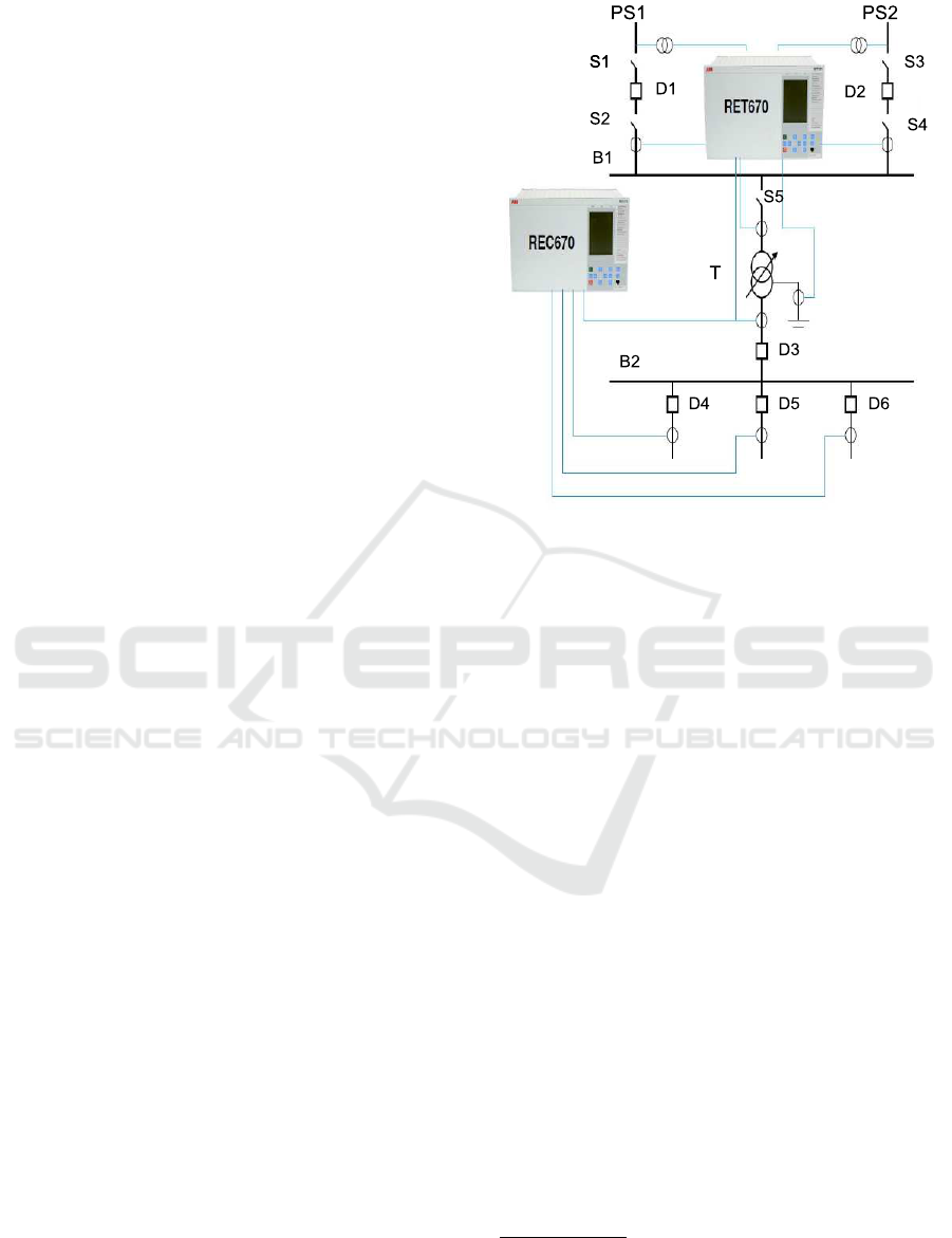
Figure 2: Bus Feeder System and Power Supply (Ltd,
2010).
4 APPLICATION TO A
SUBSTATION
As application, it is made the modelling, monitoring
and control of the EPS represented in Figure 2 by
its single line diagram. It is a substation composed
of two buses, [B
1
and B
2
], six circuit breakers [D
1
,
D
2
,··· ,D
6
], five disconnectors [S
1
,···, S
5
], one trans-
former and three energy consumers.
First of all, considering the substation de-
energized [i.e. the switch-disconnectors and circuit-
breaker assemblies are all disconnected or open].
With this, the following procedure
1
can be proposed
to energize the buses B
1
and B
2
:
1. To power on the Bus B
1
via PS
1
, must be given
priority to close the disconnecting switches S
1
and
S
2
and after these the circuit breaker D
1
must be
closed;
2. To power on the Bus B
1
via PS
2
, must given pri-
ority to close the disconnecting switches S
3
and
S
4
and after these the circuit breaker D
2
must be
closed;
3. To power on the Transformer T after the Bus B
1
is on, it must be given priority to close the discon-
nect switch S
5
. So after that, the circuit breaker D
3
1
Any procedure proposed must be in agreement with lo-
cal standards and aligned with the concessionary that holds
the formal authorization to distribute electricity in the re-
gion in that the substation is installed.
Electric Power System Operation: A Technique to Modelling, Monitoring and Control via Petri Nets
653
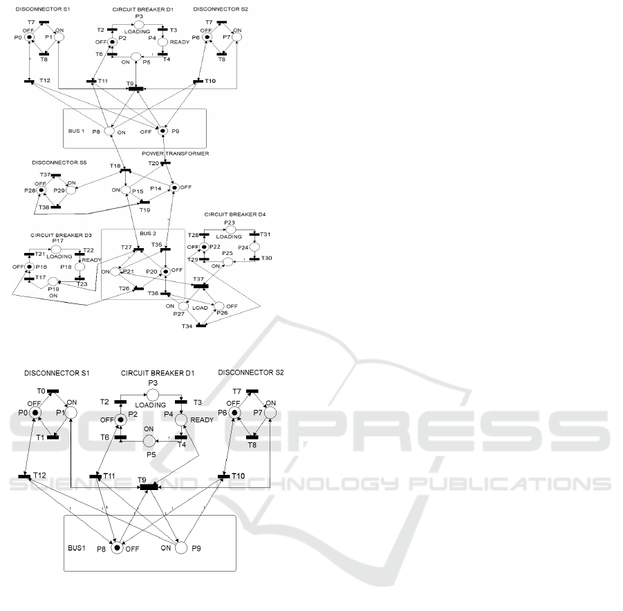
Figure 3: Substation Free Behaviour PN Modeling.
Figure 4: PS
1
Free Behaviour PN Modeling.
can be closed and consequently the bus B
2
will be
on;
4. To energize some electric loads after bus B
2
is on,
one circuit breaker must switch on D
4
to D
6
with-
out setting an order of priority;
5. The procedure for shutdown the substation must
obey an inverse prioritization order those done for
startup it [i.e. first of all, it must disconnect the
loads by switching off D
4
to D
6
, then isolating
the bus B
2
through D
3
, following with the de-
energizing of the transformer through S
5
and so
on];
4.1 Free Behavior Modeling for
Substation
Some specifications are adopted for modeling of the
substation as following. The disconnect switches
have two possible states: (i) the connected state; and
(ii) the disconnected state. The circuit breakers have
4 states: (i) the Off state; (ii) Carrying the Spring
State; (iii) ready to go Into Operation State; and the
On State. For this modeling, abnormal conditions of
the equipment are not considered [for instance, the
broken state]. The buses also are represented by two
states: (i) de-energized; and (ii) energized.
The presence of the token depicts the current state
of the equipment. For instance, considering a discon-
nect switch where P
1
is the state that symbolizes when
it is disconnected and P
2
the state representing when
it is connected, then if a token is in P
2
it represents
that the disconnect switch is closed, otherwise [token
in P
1
] it is open.
In Figure 3, a summarized version of the free be-
havior for the substation presented in Figure 2 is pre-
sented. The substation Petri net model consists of an
input PS
1
composed of two disconnect switches S
1
and S
2
and a circuit breaker D
1
, followed by the rep-
resentation of the input bus B
1
. After this, there is
the model of the disconnect switch (S
5
), responsible
for energizing the primary winding of the transformer.
To the right side of S
5
model is the representation of
the possible states of the power transformer. In the
bottom of the Petri net, all of the other models are
presented: the model to the circuit breaker D
3
, the
output bus B
2
and the energizing circuit breaker of a
load D
4
.
4.2 Controller Design for Sequence
Operation
In Figure 4 is shown the Petri net model of the free be-
havior for the input PS
1
energizing the bus B
1
. This
representation does not contemplate the restrictions
for the operation of the disconnect switches and cir-
cuit breakers that affect the safe energization or shut-
down of the bus B
1
. These constraints are intimately
related to the constructive aspects of these operational
control elements. For example, the manipulation of
the disconnect switches must not be carried out with
the circuit-breaker switched on. Thus, the correct
way to energize the bus B
1
is closing the disconnect
switches S
1
and S
2
and after that close the circuit
breaker D
1
.
For the energizing and de-energizing operation of
the PS
1
, it is necessary to compute a controller that
can restrict some actions of the free behavior model.
ICINCO 2022 - 19th International Conference on Informatics in Control, Automation and Robotics
654
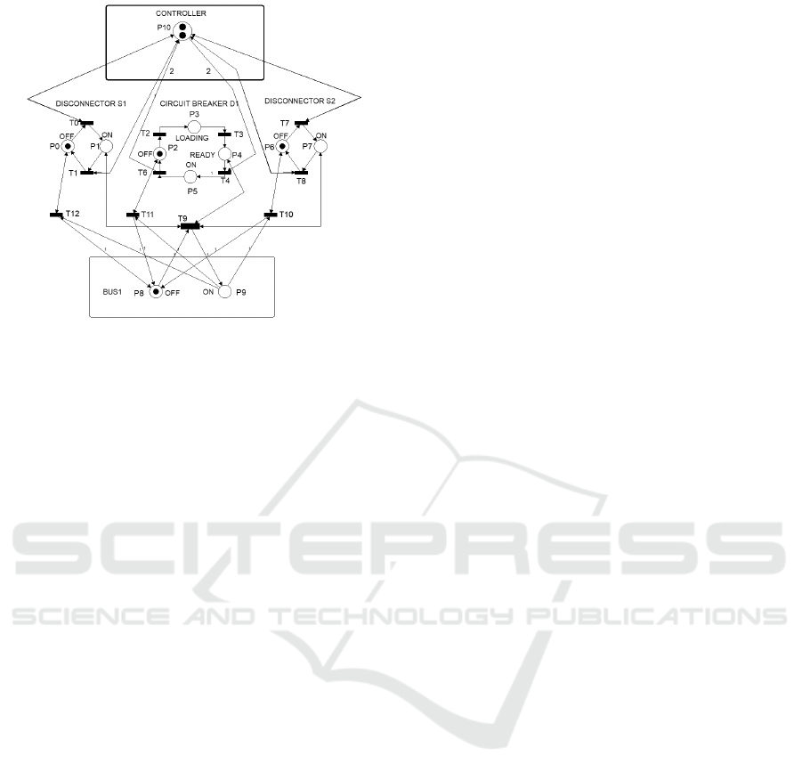
Figure 5: PS
1
System Control Modeling Using PN.
For this, it is necessary to specify the controller ac-
tions to guarantee the correct sequence of events fir-
ing. A control system is presented in Figure 5. The
control specifications are represented by a set of linear
equations where their variables represent the marking
of the controlled places. The constant on the other
side of the equation will mean that the controlled
places will form a place invariant with the controllers
[see Equation(12)].
To specify the controllers, it is necessary to find
the incidence matrix B
c
of these places and also their
initial marking M
c
(0). The incidence matrix B
c
is ob-
tained from both the control specifications and the in-
cidence matrix of the original Petri net.
From Figure 5, the constraints on this feeder can
be found by making the following considerations with
respect to feeder free behavior model PS
1
:
1. If the current state of the circuit-breaker is closed
[i.e., P
5
with marks], it forces that the current
states of the disconnect switches are also on states
[P
1
and P
7
];
2. Generating equation P
5
+ P
1
+ P
7
= 3;
3. If the current state of one of the connect switches
is opened [i.e., P
0
or P
6
with marks] the breaker
can not to close [P
5
= 0];
4. Generating equation P
5
+ P
0
+ P
6
= 1;
Adding the two equations above one can get
2P
5
+ P
0
+ P
1
+ P
6
+ P
7
= 4
and consequently
L = [1, 1, 0, 0, 0, 2, 1, 1, 0, 0].
With L and the incidence matrix, the weights of
the arc that interconnects the controller with the tran-
sitions of the original Petri net are obtained from
C B = −L B = [±1, ±1, 0, 0, −2, 2, ±1, ±1, 0, 0].
The determination of the initial marking of the
controller is obtained through Equation(12). With the
value of the initial marking of the controlled places
[i.e., P
0
, P
1
, P
5
, P
6
and P
7
], the vector L and the con-
stant K, K = 4. Found: M
c0
= 2. With this informa-
tion the Petri net of Figure 5 is drawn.
The terms represented by ± correspond to the
nonzero position in the vector L that resulted in zero
in the calculation of Equation(12). In the forma-
tion of the controlled Petri net, these positions will
be represented by autoloop. see Figure 5. The au-
toloop present between the transitions of the connect
switches models and the controller allows these tran-
sitions to fire without changing the controller mark-
ing. This condition releases the models of the connect
switches to move from the off state (P
0
and P
7
with to-
kens) to on state (P
1
and P
8
with tokens) freely. When
the model representing the circuit breaker goes to the
on state (P
5
with mark), the T
4
transition removes two
marks from controller (P
10
). The controller place, P
10
,
without marking inhibits firing of the transitions be-
longing to the switch models (T
0
, T
1
, T
7
, and T
8
). This
condition (P
10
without tokens) keeps the model of the
disconnect switches in the state that were before the
T
4
transition firing.
In agreement with the constraints imposed to de-
termine the controller, the following sequence of
events are possible: T
0
T
7
T
2
T
3
T
4
representing the on
states of the switches, breaker and bus(P
1
, P
5
, P
7
and
P
9
with marks) and another sequences are T
5
T
1
T
8
or T
5
T
8
T
1
representing the states off the disconnect
switches, circuit breaker and bus (M
0
). In relation
to the bus, it already loses the on status as soon as
T
5
fires since the model contemplates the way the
switches and circuit breakers are physically intercon-
nected(series association).
4.3 Development of the Monitor
In Figure 3 is shown the Petri net model for the in-
put power supply PS 1 of the sub-station presented
in Figure 6. A new transition T
5
has been inserted
to represent a failure event. This event connects both
the place that represents the Ready Circuit Breaker
Status and the place that represents off State Circuit
Breaker Status. Thus, T
5
emulates possible problems
that may appear on the circuit breaker, such as loss of
elastic characteristics of the spring assembly, jammed
or worn contacts, etc. Consider T
5
be uncontrollable
and observable means that the controller can not in-
tervene in its firing but the monitor alarms if it comes
to fire.
So, given the Incidence matrix B of the Petri net of
Figure 6 and knowing that when specifying a monitor
Electric Power System Operation: A Technique to Modelling, Monitoring and Control via Petri Nets
655
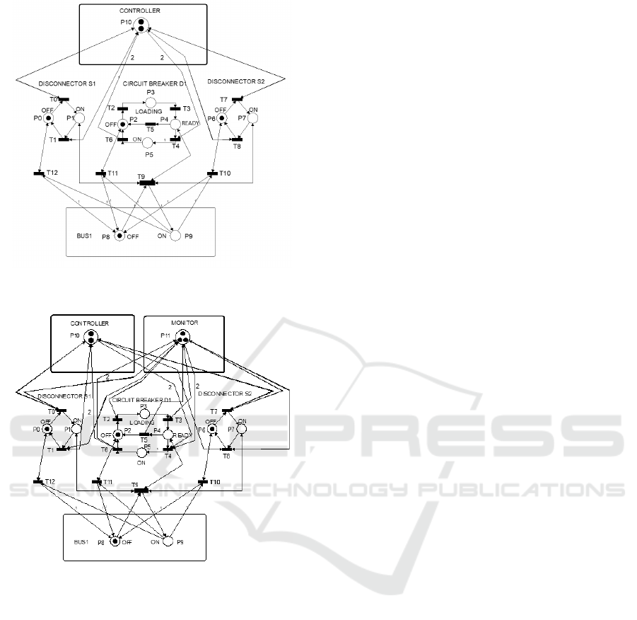
Figure 6: PN Model for PS1 With Uncontrolled and Ob-
servable Transition.
Figure 7: Structure of a Monitor for PS1 With Failure Tran-
sition.
for the main places those represents S
1
, S
2
and D
1
the
vector L will be.
L =
1, 1, 1, 1, 1, 1, 1, 1, 0, 0, 1
And applying the condition for monitoring in the
Equation(10). It is determined that the weight of the
arcs between the monitor place and the Perti net will
be:
B
m
=
±1±1 ±1±1−2 2±1±1±1±1 00±1
Transition T
5
is occupying the last column of the inci-
dence matrix B. It is a non-controllable transition and
therefore the monitor will not be able to intervene in
its fire. This condition eliminates in the computation
of vector B
m
the arc that will link the place monitor
to the transition T
5
. That way, the monitor will know
if the transition T
5
has fired but it does not interfere
in your fire. The last field of the B
m
vector loses the
value -1 and retains the +1 value. See B
m
below.
B
m
=
±1±1 ±1±1−2 2±1±1±1±1 001
The initial marking for the monitor will be ob-
tained through Equation(10). Thus, the new Petri net
is shown in Figure 7
By analyzing the Petri net of Figure 7 are ex-
tracted the following informations:
1. The firing of all controllable transitions remains
invariant between the monitored and monitor
places.
2. The fire of the uncontrolled transition causes the
breaking of the invariant place, allowing the iden-
tification of the failure.
3. The number of monitor marks expresses the num-
ber of times the failure occurred.
4. The occurrence of the fault causes loss of control
by the controller P
10
.
5. The Monitor does not interfere in the actions of
the controller.
5 CONCLUSION
The approach adopted in this work proved to be a
tool capable of expanding a Petri net to an enlarged
Petri net without, however, interfering with the mark-
ing of the original one. The Invariant Place property
of the Petri net, when forced, such a place acquires
characteristics that allow monitoring, controlling and
diagnosing plants just like an EPS. By marking the
place added to the original Petri net, it is possible to
associate it with a system operating state and iden-
tify an abnormal operating condition (monitoring fea-
ture) or allow it to intervene in the system with a con-
trol action (control feature ). Thus, the use of Place-
Transition Petri nets proved to be very useful in mod-
eling, monitoring and controlling the operation of an
EPS, making such tasks simpler, elegant and effec-
tive.
It is found that an inserted place gains the property
of monitoring the original Petri net when the place
monitor has the same total number of marks of the
monitored model. The divergence between the mon-
itor marking and the monitored model marking is a
flag that occurs something wrong.
When it is imposed, the sum of the markings of the
place inserted with the markings of the original Petri
net is equal to a predefined constant k. This place
gains ownership of controlling Petri net actions from
constraints imposed. This new property is acquired
ICINCO 2022 - 19th International Conference on Informatics in Control, Automation and Robotics
656

by the added place, via the geometric approach cre-
ated using the free model for a circuit breaker and a
disconnector. Thus, it was verified that the inserted
place was able to control the sequence of those mod-
els that represent this equipment validating the model.
ACKNOWLEDGEMENTS
This work was partially supported by CAPES
(Coordenac¸
˜
ao de Aperfeic¸oamento de Pessoal de
N
´
ıvel Superior).
REFERENCES
Amini, S., Pasqualetti, F., Abbaszadeh, M., and Mohsenian-
Rad, H. (2019). Hierarchical location identification of
destabilizing faults and attacks in power systems: A
frequency-domain approach. IEEE Transactions on
Smart Grid, 10(2):2036–2045.
Bin, S. Y., Ping, C. Y., and Zhan, B. (2015). Fault diagnosis
for power system using time sequence fuzzy Petri net.
In 3rd International Conference on Mechanical Engi-
neering and Intelligent Systems (ICMEIS), volume 1,
pages 729–735.
Cassandras, C. G. and Lafortune, S. (2009). Introduction to
discrete event systems. Springer Science & Business
Media.
David, R. and Alla, H. (1994). Petri nets for modeling of
dynamic systems - a survey. Automatica, 30(2):175–
202.
Dideban, A. and Alla, H. (2009). Feedback control logic
synthesis for non safe Petri nets. IFAC Proceedings
Volumes, 42(4):942 – 947.
Fendri, D. and Chaabene, M. (2019). Hybrid Petri net
scheduling model of household appliances for optimal
renewable energy dispatching. Sustainable Cities and
Society, 45:151 – 158.
Giua, A. (1992). Petri Nets as Discrete Event Models for
Supervisory Controls. PhD thesis, Dept. Electrical
Computer and Systems Engineering, Rensselaer Poly-
technic Institute.
Grainger, J. J. and Stevenson Jr., W. D. (1994). Power Sys-
tem Analysis.
Holloway, L. E., Guan, X., and Zhang, L. (1996). A gen-
eralization of state avoidance policies for controlled
Petri nets. IEEE Transactions on Automatic Control,
41(6):804–816.
Komenda, J., Lahaye, S., Boimond, J.-L., and van den
Boom, T. (2018). Max-plus algebra in the history of
discrete event systems. Annual Reviews in Control,
45.
Krogh, B. H. and Holloway, L. E. (1991). Synthesis of feed-
back control logic for discrete manufacturing systems.
Automatica, 27(4):641–651.
Lin, W., Luo, J., Zhou, J., Huang, Y., and Zhou, M. (2016).
Scheduling and control of batch chemical processes
with timed Petri nets. In IEEE International Confer-
ence on Automation Science and Engineering (CASE),
pages 421–426.
Ltd, A. (2010). Abb special report iec 61850. Technical
report.
Moody, J. O. and Antsaklis, P. (2000). Petri net supervisor
for des with uncontrollable and unobservable transi-
tion. IEEE Transactions Automatic Control, Man, and
Cybernetics, Part B (Cybernetics), 45(3):462–476.
Murata, T. (1989). Petri nets: Properties, analysis and ap-
plications. Proceedings of IEEE, 77(4):541–580.
Papadopoulos, C. T., Li, J., and O’Kelly, M. E. J. (2019).
A classification and review of timed markov models
of manufacturing systems. Computers and Industrial
Engineering, 128:219 – 244.
Souza, M., Lima, E., and Cerqueira, J. (2016). Electric
power system operation: A Petri net approach for
modelling and control. In 13th International Con-
ference on Informatics in Control, Automation and
Robotics, volume 1, pages 477 – 483.
Tekiner-Mogulkoc, H., Coit, D. W., and Felder, F. A.
(2012). Electric power system generation expansion
plans considering the impact of smart grid technolo-
gies. International Journal of Electrical Power & En-
ergy Systems, 42(1):229 – 239.
Vescio, G., Riccobon, P., Grasselli, U., and Angelis, F. D.
(2015). A Petri net model for electrical power sys-
tems operating procedures. In Annual Reliability and
Maintainability Symposium (RAMS), pages 1–6.
Weiss, T. and Schulz, D. (2015). A generic optimiza-
tion tool for power plant dispatch and energy storage
system operation. In 50th International Universities
Power Engineering Conference (UPEC), pages 1–6.
Wu, X., Tian, S., and Zhang, L. (2019). The internet
of things enabled shop floor scheduling and process
control method based on Petri nets. IEEE Access,
7:27432–27442.
Zhou, M. C., Dicesare, F., and Rudolph, D. L. (1992). De-
sign and implementation of a Petri net based supervi-
sor for a flexible manufacturing system. Automatica,
28(6):1199 – 1208.
Electric Power System Operation: A Technique to Modelling, Monitoring and Control via Petri Nets
657
