A Computer Vision Approach to Predict Distance in an Autonomous

Vehicle Environment

Giuseppe Parrotta, Mauro Tropea

and Floriano De Rango

DIMES Department, University of Calabria, via P. Bucci 39c, 87036 Rende (CS), Italy

Keywords:

Autonomous Vehicles, Autonomous Guide, Computer Vision, Interpolation Technique, Machine Learning.

Abstract:

Autonomous vehicle (AV) is a kind of intelligent car, which is mainly based on the computer and sensor

system inside the car to realize driverless guide. The AVs are cars that recognize the driving environment

without human intervention, assess the risk, plan the driving route and operate on their own. These vehicles are

integrated with a series of sensors and other devices and software like automatic control, artiﬁcial intelligence,

visual computing in order to be able to perform driving inside a road. Calculate the correct distance between

vehicle and objects inside its trajectory is important to allow an autonomous guide in safety. So, in this paper

we describe our proposal of predicting this distance in a real scenario through an on-board camera and with

the support of rover, arm platforms and sensors. The proposal is to use an interpolation technique that permits

to predict distance with a good accuracy.

1 INTRODUCTION

An autonomous car, also known as an autonomous ve-

hicle (AV), driverless car or robo-car, is a vehicle ca-

pable of detecting the surrounding environment and

moving through it safely with or without human in-

tervention. By deﬁnition, autonomous vehicles are

able to update their maps based on sensor inputs, al-

lowing vehicles to keep track of their position even

when conditions change or when entering environ-

ments unknown to them (Talavera et al., 2021), re-

alizing driverless guide (Mariani et al., 2021). The

research on vehicular networks is most promising in

the last years approaching with the use of the mod-

ern techniques based on artiﬁcial intelligence and ma-

chine learning paradigms but also the Cloud, Edge

and Fog computing that aiding vehicles in the com-

putation processes. Moreover, the use of Internet of

Things (IoT) in the vehicular environment is another

important ﬁeld of study object of different works in

literature (De Rango et al., 2022), (Tropea et al.,

2021). Many studies regard also routing (Fazio et al.,

2013), emission issues (Santamaria et al., 2019a),

channel modeling (Fazio et al., 2015).

Intelligent vehicles have a series of intelligent

agents integrated on multi-sensors that are based on

https://orcid.org/0000-0003-0593-5254

https://orcid.org/0000-0003-4901-6233

the perception and modeling of the environment, lo-

calization and construction of maps, path planning,

decision-making and motion control. An important

aspect in the AV context is also related to coordination

of group of vehicles forming that so called ”platoon”.

So, opportune coordination protocols have to be stud-

ied as shown in (Palmieri et al., 2019), (De Rango

et al., 2018) and then the execution of multiple tasks

for vehicles that operate in group (Palmieri et al.,

2018).

As it is possible to view in Figure 1 the main op-

erational functions performed by an AV are depicted

and described in the following. The ”perception and

modeling of the environment” module is responsible

for the perception of the structure of the environment,

relying on the support of multiple sensors and cam-

eras, and thus building a model of the surrounding

environment. The template attaches a list of moving

Figure 1: Intelligent vehicles operations.

348

Parrotta, G., Tropea, M. and De Rango, F.

A Computer Vision Approach to Predict Distance in an Autonomous Vehicle Environment.

DOI: 10.5220/0011318400003274

In Proceedings of the 12th International Conference on Simulation and Modeling Methodologies, Technologies and Applications (SIMULTECH 2022), pages 348-355

ISBN: 978-989-758-578-4; ISSN: 2184-2841

objects, obstacles, the relative position of the vehi-

cle with respect to the road traveled, the shape of the

road etc. Finally, this module provides the environ-

ment model and the local map to the ”map localiza-

tion and construction” module with the processing of

the initial data and the data provided by vision, lidar

or radar. The ”Localization and construction of the

maps” module uses geometric knowledge in estimat-

ing the position in the map to determine the position

of the vehicle and to interpret the information from

the sensors in order to estimate the geometric loca-

tion in the global map. As a result, this module deter-

mines a global map based on the environment model

and the local map. The “path planning and decision

making” module ensures the vehicle its safe interac-

tion in accordance with the rules of safety, comfort,

vehicle dynamics and environmental context. The last

module ”Motion Control” is responsible of the vehi-

cle movement in the map considering an autonomous

guide in a real environment. So, it executes the com-

mands necessary to travel the planned route, thus pro-

ducing interaction between the vehicle and the sur-

rounding environment.

In this paper, we propose the use of an interpola-

tion technique in order to compute distance between

vehicles and objects in the scene in order to have a

good precision and accuracy in the performed mea-

surements. First of all, throughout the use of machine

learning approach, the vehicle is able to identify the

object in front of it through the use of an on-board

camera, and then, on the basis of the proposed tech-

nique it is able to compute and predict with a good ac-

curacy the distance between itself and the recognized

object in its trajectory. The conducted experiments

are shown and the opportune considerations are ex-

plained in the rest of the paper. The structure of the

paper is the following: Section 2 described brieﬂy the

main literature on autonomous vehicles; Section 3 de-

scribes the concept of obstacles recognition in the ref-

erence context; Section 4 shows the main conducted

experiments and the relative results; ﬁnally, the paper

ends with the conclusions provided in Section 5.

2 RELATED WORK

The future car will be able to guide in every con-

text without human intervention. The research in

these years is studying different mechanisms in or-

der to make the autonomous guide a real experi-

ence in a near feature. Six different levels of au-

tonomy are been individuated and nowadays the re-

search effort is related to last level, the level number 5,

that aims to make the guide completely autonomous

thanks to the great progress in technology, robotic and

electronic (Aut, 2022). Autonomous vehicles scan

the environment with techniques such as radar, lidar,

GNSS, and machine vision through on-board camera

(Jim

enez et al., 2018). Advanced control systems in-

terpret the information received to identify appropri-

ate routes, obstacles and relevant signs. So, in liter-

ature a lot of works exist that deal with this interest-

ing topic and many of these provide overview on dif-

ferent aspects concerning AVs, their communication

type (Duan et al., 2021), and on the impact that the

AVs will have in our cities (Duarte and Ratti, 2018).

The awareness of the environment is due, other than

different sensors, to camera/cameras placed in front

of the vehicle. A monocular vision for extracting im-

age features used for calculating pixel distance is pro-

posed in (Aswini and Uma, 2019).

In (Salman et al., 2017) the authors propose the

use of stereo camera to measure the distance of an

object and so avoiding obstacles in the navigation of

autonomous vehicles. Their measures are based on

angular distance, distance between cameras, and the

pixel of the image and using the trigonometry for

computing the object distance. In (Park and Choi,

2019) the authors present the detailed design and im-

plementation procedures for an advanced driver as-

sistance system, called ADAS, based on an open

source automotive open system architecture called

AUTOSAR. The main purpose of the work is to pro-

pose, in this type of architecture, a collision warning

system able to detect obstacles on the road. They pro-

vide a set of experimental results that can help de-

velopers to improve the overall safety of the vehic-

ular system. For their experiments actual ultrasonic

sensors and light-emitting diodes (LEDs) connected

to an AUTOSAR evaluation kit has been used with

the integration of a virtual robot experience platform

(V-REP). In (Kim et al., 2021) the authors deal with

the safety issues in an autonomous vehicle system.

They refer to Mobileye, a company that proposed the

RSS (responsibility-sensitive safety) model to prevent

the accidents of autonomous vehicles (Shashua et al.,

2018). This RSS model is a mathematical model that

aids to ensure safety trying to determine whether an

autonomous vehicle is at fault in an accident propos-

ing a safe distance. They propose a mechanism to cal-

culate safe distance for each velocity through the use

of a camera, in particular they calculate lateral and

longitudinal safe distance.

In (El-Hassan, 2020) the authors propose a small-

size prototype of an autonomous vehicle equipped

with low-cost sensors driving on an artiﬁcial road

structure. They have tested their experiments using

as obstacles a toy vehicle placed on the road traveled

A Computer Vision Approach to Predict Distance in an Autonomous Vehicle Environment

349

by the prototype. The experiments have shown that

it is able to detect the obstacle and turn to avoid col-

lision remaining on the correct road lane. In (Philip

et al., 2018) the authors study and analyze a smart

trafﬁc intersection management application for auto-

mated vehicles by the point of view of the effect of de-

lay–accuracy trade-off in real-time applications. The

research is pushing also for autonomous electrical ve-

hicles in order to pay attention to the green and energy

consumption with many works that deal with these

topics (De Rango et al., 2020). An overview of the

enabling technology and the architecture of the Cog-

nitive Internet of Vehicles for autonomous driving is

presented in (Lu et al., 2019).

On the basis of the considered literature, in this

work we want to propose an approach to compute and

predict obstacles distance based on on-board camera

that uses an interpolation mechanism able to guaran-

teeing a good accuracy. The experimentation is done

with a real rover equipped with a camera and an ultra-

sonic sensor used for validate the distance calculated

through the on-board camera.

3 OBSTACLES RECOGNITION

In general, in a driving environment, we are inter-

ested in static/dynamic obstacles, road markings, road

signs, vehicles and pedestrians. Consequently, object

detection and tracking are the key parts of environ-

mental perception and modeling. The goal of vehicle

tracking and mapping is to generate a global map by

combining the environmental model, a local map and

global information. In autonomous driving, vehicle

tracking is to estimate the geometry of the road or lo-

cate the vehicle relative to the roads in the conditions

of known maps or unknown maps. Hence, vehicle lo-

cation refers to estimating the road shape and location

by ﬁltering, transforming the vehicle’s location into a

coordinate frame.

In general, the perception and modeling of the sur-

rounding environment takes place in this way: [1.] the

original data is received and collected by the various

sensors; [2.] the different features are extracted from

the original data such as the color of the road (or ob-

jects), the stripes and the outlines of the buildings; [3.]

semantic objects are recognized thanks to the use of

classiﬁers and consist of stripes, signals, vehicles and

pedestrians; [4.] the driving context and the position

of the vehicle are deduced.

Sensors used for the perception of the surround-

ing environment are divided into two categories: ac-

tive and passive. Active sensors include lidar, radar,

ultrasound and radio, while commonly used passive

sensors are infrared and visual cameras (Wang et al.,

2022). The visual analysis of complex scenes, where

the essence of the objects present cannot be cap-

tured by purely geometric models, is one of the most

difﬁcult challenges in present and future research,

greatly used in video surveillance systems (Santa-

maria et al., 2019b). Robotic perception is related to

many applications in robotics where sensory data and

artiﬁcial intelligence/machine learning (AI/ML) tech-

niques are involved.

Nowadays, most robotic perception systems use

machine learning (ML) techniques which can be in

the form of unsupervised learning or supervised clas-

siﬁers using features or deep learning neural networks

(e.g., convolutional neural network (CNN)) or even a

combination of multiple methods. Each object pro-

cess receives image data (pixels) from the video sec-

tion of the vision system and continuously generates

a description of the assigned object. In the ﬁrst phase,

the extraction of the features, the groups of pixels are

combined into features, such as edges or corners. Fea-

ture extraction can be supported by the next higher

level in the processing hierarchy, the 2D object level.

Here, knowledge of the appearance of speciﬁc phys-

ical objects is used to generate hypotheses about the

nature of the object itself and the expectations of the

features that should be visible and where they should

appear in the image. Many features can be detected

but they differ on the basis of the distance of the ob-

ject. Greater is this distance lesser deﬁned are the

edge of the image. The study of the structure of an

image is essential to understand how to apply the al-

gorithms that allow to process and interpret the image.

The extraction of the reference points is carried out

through an edge detection algorithm. In order to rec-

ognize the image in the scene, in this paper, we have

used a machine learning approach. So, we are able to

identify the object in front of the vehicle and through

the use of the camera on-board we are able also to

compute the correct distance from the recognized ob-

ject. In the following section, we will describe the

conducted experiments explaining in detail the envi-

ronment and the scene considered for the tests.

4 EXPERIMENTATION

The purpose of the experimental work is to trace

the actual value of the distance between the obsta-

cle placed in front of the rover (model car, see Fig-

ure 2), managing to obtain this data exclusively with

the aid of the video camera (with which the model

car is equipped) and with the support of the instru-

ments offered by OpenCV computer vision libraries

SIMULTECH 2022 - 12th International Conference on Simulation and Modeling Methodologies, Technologies and Applications

350

and APIs for programming TensorFlow neural net-

works. Thanks to this it was possible for each object

placed in front of the camera to recognize and identify

each object with an average accuracy of 70% and to

predict the value of the distance of the obstacle from

the rover.

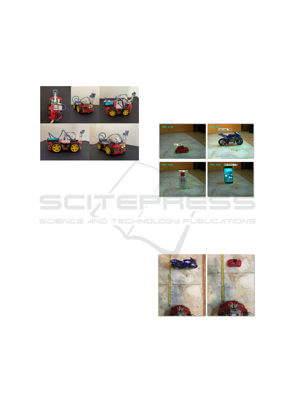
Figure 2: Rover used for experiments.

4.1 Environment Description

Regarding used hardware, the rover, the Arduino

UNO rev3 and Raspberry Pi4B platforms specially

mounted on the body of a model car equipped with

4 motors that provide traction were used for the de-

velopment and implementation of the embedded au-

tonomous driving system, see Figure 2. From soft-

ware side, instead, the algorithms have been de-

veloped for Arduino through its IDE and the pro-

gramming language Wiring, derived from C and C

++. While for Raspberry, based on the Linux Rasp-

bian operating system, the software was developed in

Python with the help of the Mu IDE. The recognition

algorithms were developed using the OpenCV soft-

ware library and TensorFlow models.

For the rover, being equipped with a camera and

an ultrasonic proximity sensor, a recognition algo-

rithm was developed to be able to identify the ob-

jects in front of them and calculate their distance.

This algorithm was developed in Python and with the

support provided by the OpenCV and TensorFlow li-

braries. The video stream is ﬁrst initialized by re-

ceiving the images supplied by the camera as input.

The captured frame is normalized and resized with

the support of computer vision (offered by OpenCV),

after which object recognition is performed by an al-

ready trained artiﬁcial intelligence in charge of object

recognition only. The tensor outputs the object name

and the recognition accuracy percentage. This infor-

mation is returned to the screen with OpenCV which

also builds the box that frames the object. Further-

more, when the object is recognized, the script cal-

culates the distance value by means of the sensor and

returns this value to the screen as before with the help

of OpenCV. At the end of the analysis of this frame,

we move on to the next one and repeat this process.

The user can also decide to stop the execution of the

algorithm at any time. In the case of object is recog-

nized, this will automatically be surrounded by a box

that delimits the area covered by it and the name and

the percentage of accuracy in the recognition will be

indicated. Pictures in Figure 3 are shown as an exam-

ple of how this recognition system works.

Figure 3: Example of how the recognition algorithm identi-

ﬁes the different objects in the space and indicates the pos-

sible name and percentage of accuracy.

First of all, it was necessary to calibrate the con-

sidered scene thanks to the ultrasonic sensor the rover

is equipped with and which provided a very true and

precise estimate of the distances that are detected, see

Figure 4.

Figure 4: Example of measures performed by sensor and

veriﬁed by the use of a rule in order to compute the preci-

sion.

The measurements made by the sensor were ver-

iﬁed with the aid of a rule to certify their accuracy.

On the basis of this, a template was built which con-

A Computer Vision Approach to Predict Distance in an Autonomous Vehicle Environment

351

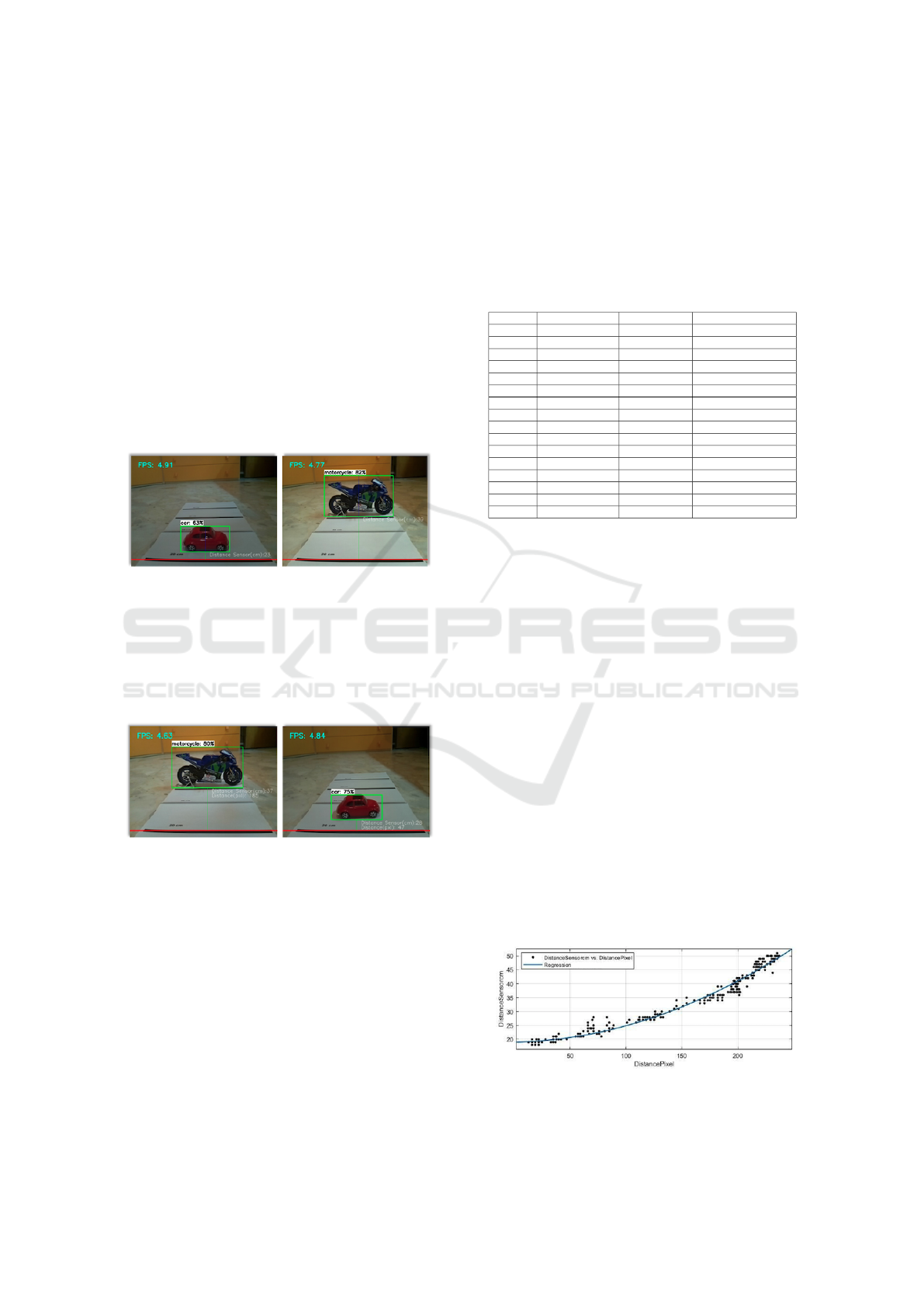
sists of a print with lines separated from each other

by 10 centimeters which was useful for having at this

stage some real and concrete references of the mea-

surements at the time of future sampling. Then, a ref-

erence in the scene was placed and highlighted with a

red line at a distance of 20 centimeters from the front

of the car. This distance was considered as safety dis-

tance to avoid collisions between the rover and ob-

stacles present in the trajectory. For each frame and

for each recognized object (highlighted by its box)

we have identiﬁed the exact center of the rectangle,

called ”C”, that deﬁnes a characteristic point of a sin-

gle object, see Figure 5. Once this reference point

has been identiﬁed, it is projected on the basis of the

relevant object identiﬁcation box, and will be deﬁned

hereinafter as ”center of gravity”, see Figure 6.

Figure 5: The center ”C” is projected on the lower edge of

the frame to identify the characteristic point called ”center

of gravity”.

Thus, having found for each object its ”center

of gravity” it was possible to estimate the distance

in pixels between that point and the red safety line

placed in the scene.

Figure 6: The ”center of gravity” permits to estimate the

distance in pixel between the object and the red line (dis-

tance of security).

4.2 Experimental Results

On the basis of the distance obtained in pixels and that

measured by means of the ultrasonic proximity sen-

sor, a Python script was developed which collects and

saves the aforementioned data for each frame in an

Excel sheet useful for subsequent analysis. First, the

Excel ﬁle is created which indicates in which columns

the data must be entered and the label assigned for

each. In order to produce and collect data, by means

of the script, various objects were placed in front of

the rover and for each of these it was possible to de-

ﬁne an effective distance measured in centimeters,

which we will call ”Distance Sensor cm” and a dis-

tance from the ”center of gravity” expressed in pixels,

deﬁned as “Distance Pixel”. In Table 1 some exam-

ples from sampling of an object of type ”cell phone”

are reported.

Table 1: Examples taken from sampling of an object of type

”cell phone”.

Date Object Detected Distance Pixel Distance Sensor (cm)

19:10:40 cell phone: 73% 37 19

19:10:40 cell phone: 67% 35 19

19:10:41 cell phone: 64% 33 19

19:10:41 cell phone: 66% 25 19

19:10:41 cell phone: 64% 22 19

19:10:41 cell phone: 66% 22 18

19:10:42 cell phone: 68% 19 18

19:10:42 cell phone: 67% 16 20

19:10:42 cell phone: 68% 19 18

19:10:43 cell phone: 67% 22 18

19:10:43 cell phone: 67% 19 18

19:10:43 cell phone: 66% 19 18

19:10:43 cell phone: 66% 22 19

19:10:43 cell phone: 67% 22 19

Hence, the need to ﬁnd the mathematical relation-

ship by means of a function between the ”distance in

centimeters” data (which is remembered to be the one

measured with the sensor) and the ”distance in pix-

els” data (pixels between the center of gravity and

the safety line). The support offered by Matlab, and

in particular its ”Curve Fitting” application helped

in this case. The data was then imported into the

Workspace with the ”ImportData” function in 2 col-

umn vectors identiﬁed by the labels ”DistancePixel”

and ”DistanceSensorCm”. At this point, given these

vectors to ”Curve Fitting”, it was possible to iden-

tify the resulting polynomial interpolation function of

grade 2:

f (x) = p

· x

+ p

· x + p

(1)

where p

assumes the following values: p

0.0005112, p

= 0.008219, p

= 18, 96.

The value of the function f (x) represents the value

of the distance in centimeters calculated varying the

values of x. In this case, these values represent the

values of the distance expressed in pixels.

Figure 7: Quadratic regression function.

Following the function thus obtained from the re-

SIMULTECH 2022 - 12th International Conference on Simulation and Modeling Methodologies, Technologies and Applications

352

lationship between the collected data, it was possi-

ble to add to the script a function for calculating this

distance called ”InterpolationDistance”. For this rea-

son, a second data collection was proposed with the

methodology indicated above and it was possible to

relate the distance in pixels and the measurement of

the distance obtained with the interpolation function,

see Figure 7. For completeness and comparison for

each pair of data, the distance value calculated thanks

to the sensor was also taken into account as a veriﬁ-

cation value. What was obtained is summarized in an

extract from the sampling reported in Table 2.

Table 2: Extract of the sampling on a ”cell phone” object

where the distance value was calculated with the interpola-

tion function.

Date Object Detected Distance Pixel Distance Sensor (cm) Interpolation Grade 2

19:11:15 cell phone: 83% 126 28 28,1114052

19:11:15 cell phone: 82% 126 28 28,1114052

19:11:16 cell phone: 83% 126 28 28,1114052

19:11:16 cell phone: 82% 126 28 28,1114052

19:11:16 cell phone: 83% 126 28 28,1114052

19:11:16 cell phone: 82% 126 28 28,1114052

19:11:17 cell phone: 83% 126 29 28,1114052

19:11:17 cell phone: 83% 128 29 28,3875328

19:11:17 cell phone: 83% 130 29 28,6677500

19:11:17 cell phone: 83% 128 29 28,3875328

19:11:17 cell phone: 81% 132 30 28,9520568

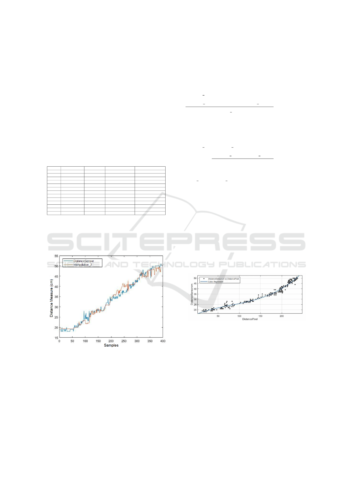
From the so obtained data it was possible to com-

pare the value of the distance calculated with the aid

of the sensor and that calculated with the interpolation

function of grade 2, see Figure 8.

Figure 8: Blue curve highlights the distance values com-

puted by sensor while the red curve highlights the distance

values computed with the interpolation function.

Therefore, it can be seen from Figure 8, where the

distance measurement for each sample is related, that

the functions called ”distanceSensor” and ”Interpola-

tionGrade2” are relatively close and close in identify-

ing the actual distance of the object. However, it is

noted that in some intervals, due to possible errors in

the sampling or in the provided estimation, the two

functions settle on different values. Hence, the need

to calculate the percentage error between the results

produced by the two functions. For each sample the

error was calculated in this way:

error percentage =

|sensor value − interpolation value|

sensor value

∗ 100(%) (2)

Lastly, an average of the error was calculated over

the whole sample:

error percentage average =

∑

error percentage value

samples

∗ 100(%) (3)

We have obtained a value of:

error percentage average = 3, 76%. For the

sake of completeness, it was decided to submit the

same data to a higher grade interpolation, with a

cubic regression, so as to verify whether it is more

efﬁcient and whether the consistency between the

calculated distance and that provided by the sensor

is greater than in the previous case, see Figure 9.

We proceeded in the same way seen before and the

function provided by ”Curve Fitting” is the following:

f (x) = p

· x

+ p

· x

+ p

· x + p

(4)

where p

= 3, 773e

−6

, p

= −0.000914, p

0.1536 and p

= 15.91.

Figure 9: Cubic regression function.

By applying this function to the set of data ob-

tained, it is possible to compare them to the actual

distance measurement provided by the instrument, be-

ing able to state that the distance value obtained in

this way considerably increases the error and provid-

ing wrong data as it is possible to observer in Figure

10.

4.2.1 Error Correction

In order to reduce the sensitive difference that arose

between the actual distance measurement and the one

calculated thanks to the quadratic interpolation func-

tion, it was decided to act as follows.

A Computer Vision Approach to Predict Distance in an Autonomous Vehicle Environment

353

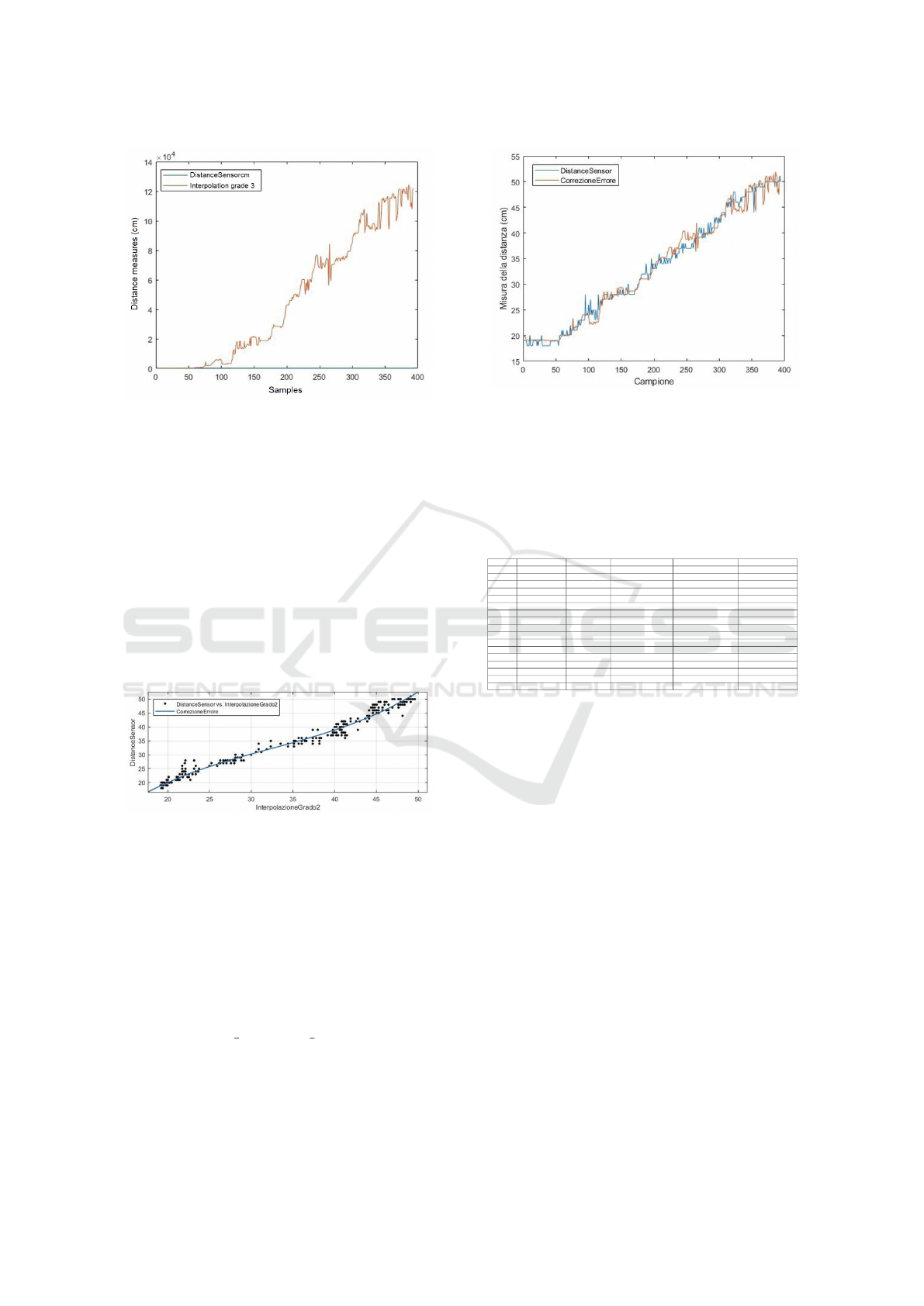
Figure 10: Blue curve highlights the distance values com-

puted by sensor while the red curve highlights the distance

values computed with the interpolation function.

Applying again the methodology seen previously,

it was possible to ﬁnd a second interpolation function

called ”error correction” of grade 3 and deﬁned as fol-

lows:

f (x) = p

· x

+ p

· x

+ p

· x + p

(5)

where p

= 0.001113, p

= −0.1083, p

= 4, 327

and p

= −32.11.

So, we have the following graphic, see Figure 11.

Figure 11: Error correction function: cubic regression.

By applying this error correction function to the

values obtained from the previous interpolation, I ob-

tain results that respond better and are closer to the

real ones calculated by means of the sensor, as can

be seen from the following graphic, Figure 12. An

extract of the sampling of ”cell phone” object is re-

ported in Table 3. Also for this second case series, the

percentage error was calculated on all the samples, in

the same way and with the same methodology seen

in the case of grade 2 interpolation, and its average

was equal to: error percentage average = 3, 2381%.

This result shows the better error percentage consid-

ering also the error correction function.

The drawback of the proposed technique is that it

is not able to guarantee a good distance prediction for

Figure 12: The blue function highlights the distance value

for each sample returned by the sensor, while the orange

function returns the same value calculated with the error

correction function. The two functions were then compared

to identify the goodness of this function.

Table 3: Extract of the sampling on a ”cell phone” object

where the distance value was calculated with the interpola-

tion grade 2 function compared with error correction func-

tion.

Date Object Detected Distance Pixel Distance Sensor (cm) Interpolation Grade 2 ERROR Correction

19:10:51 cell phone: 67% 16 19 19,2223712 18,95365633

19:10:51 cell phone: 68% 16 19 19,2223712 18,95365633

19:10:51 cell phone: 68% 13 19 19,1532398 18,85685519

19:10:51 cell phone: 68% 16 18 19,2223712 18,95365633

19:10:52 cell phone: 68% 19 19 19,3007042 19,06283251

19:10:52 cell phone: 69% 22 20 19,3882388 19,18419679

19:10:52 cell phone: 69% 28 20 19,5909128 19,46264390

19:10:52 cell phone: 71% 35 20 19,8738850 19,84552877

19:10:52 cell phone: 73% 35 21 19,8738850 19,84552877

19:10:53 cell phone: 73% 38 20 20,0104948 20,02795981

19:10:53 cell phone: 73% 38 21 20,0104948 20,02795981

19:10:53 cell phone: 71% 38 20 20,0104948 20,02795981

19:10:53 cell phone: 73% 38 20 20,0104948 20,02795981

19:10:53 cell phone: 73% 40 20 20,1066800 20,15547724

19:10:54 cell phone: 73% 38 20 20,0104948 20,02795981

19:10:54 cell phone: 71% 37 21 19,9639358 19,96595892

all the recognized objects inside the scene. It needs

different interpolation functions, one for each object

inside the scene of the vehicular environment. This

condition does not permit to have a generalized inter-

polation function able to be utilized on every object in

front the vehicle. So, in order to have a good grade of

accuracy different interpolation functions have to be

identiﬁed for each different type of recognized object

inside the vehicular scenario making the approach no

scalable and no efﬁcient to be used in real environ-

ment. A generalized approach is being under study

using different techniques based on machine learning

in order to individuate a generalized approach to be

used in each context.

5 CONCLUSIONS

In this paper we introduce the use of a technique

based on interpolation function for predicting the dis-

tance of objects in front the car equipped with a high

resolution camera. The conducted experiments have

shown the capability of computing correctly this dis-

SIMULTECH 2022 - 12th International Conference on Simulation and Modeling Methodologies, Technologies and Applications

354

tance through the use of on-board camera and how to

predict it using of an interpolation technique. The re-

sults show that the proposed approach is able to guar-

antee a good computing. For the future, it is very in-

teresting to be able of ﬁnding a generalized model that

could guarantee and efﬁcient distance estimation for

each object inside the scene. So, for this purpose we

are studying technique based on neural network ap-

proaches that promise to be more precise and reliable

and capable of guaranteeing a generalized model able

to predict object distance for different type of obsta-

cles.

REFERENCES

(2022). Automotive. https://novatel.com/industries/

autonomous-vehicles. [Online; accessed 02-March-

2022].

Aswini, N. and Uma, S. (2019). Obstacle avoidance and dis-

tance measurement for unmanned aerial vehicles us-

ing monocular vision. International Journal of Elec-

trical and Computer Engineering, 9(5):3504.

De Rango, F., Palmieri, N., Yang, X.-S., and Marano, S.

(2018). Swarm robotics in wireless distributed proto-

col design for coordinating robots involved in cooper-

ative tasks. Soft Computing, 22(13):4251–4266.

De Rango, F., Tropea, M., Raimondo, P., and Santamaria,

A. F. (2020). Grey wolf optimization in vanet to man-

age platooning of future autonomous electrical vehi-

cles. In 2020 IEEE 17th Annual Consumer Commu-

nications & Networking Conference (CCNC), pages

1–2. IEEE.

De Rango, F., Tropea, M., Serianni, A., and Cordeschi, N.

(2022). Fuzzy inference system design for promoting

an eco-friendly driving style in iov domain. Vehicular

Communications, 34:100415.

Duan, X., Jiang, H., Tian, D., Zou, T., Zhou, J., and Cao,

Y. (2021). V2i based environment perception for au-

tonomous vehicles at intersections. China Communi-

cations, 18(7):1–12.

Duarte, F. and Ratti, C. (2018). The impact of autonomous

vehicles on cities: A review. Journal of Urban Tech-

nology, 25(4):3–18.

El-Hassan, F. T. (2020). Experimenting with sensors of a

low-cost prototype of an autonomous vehicle. IEEE

Sensors Journal, 20(21):13131–13138.

Fazio, P., Sottile, C., Santamaria, A. F., and Tropea,

M. (2013). Vehicular networking enhancement and

multi-channel routing optimization, based on multi-

objective metric and minimum spanning tree. Ad-

vances in Electrical and Electronic Engineering,

11(5):349–356.

Fazio, P., Tropea, M., Sottile, C., and Lupia, A. (2015).

Vehicular networking and channel modeling: a new

markovian approach. In 2015 12th Annual IEEE Con-

sumer Communications and Networking Conference

(CCNC), pages 702–707. IEEE.

Jim

enez, F., Clavijo, M., Castellanos, F., and

Alvarez, C.

(2018). Accurate and detailed transversal road section

characteristics extraction using laser scanner. Applied

Sciences, 8(5):724.

Kim, M.-J., Yu, S.-H., Kim, T.-H., Kim, J.-U., and Kim, Y.-

M. (2021). On the development of autonomous vehi-

cle safety distance by an rss model based on a variable

focus function camera. Sensors, 21(20):6733.

Lu, H., Liu, Q., Tian, D., Li, Y., Kim, H., and Serikawa,

S. (2019). The cognitive internet of vehicles for au-

tonomous driving. IEEE Network, 33(3):65–73.

Mariani, S., Cabri, G., and Zambonelli, F. (2021). Coordi-

nation of autonomous vehicles: taxonomy and survey.

ACM Computing Surveys (CSUR), 54(1):1–33.

Palmieri, N., Yang, X.-S., De Rango, F., and Marano, S.

(2019). Comparison of bio-inspired algorithms ap-

plied to the coordination of mobile robots consider-

ing the energy consumption. Neural Computing and

Applications, 31(1):263–286.

Palmieri, N., Yang, X.-S., De Rango, F., and Santamaria,

A. F. (2018). Self-adaptive decision-making mecha-

nisms to balance the execution of multiple tasks for a

multi-robots team. Neurocomputing, 306:17–36.

Park, J. and Choi, B. W. (2019). Design and implementa-

tion procedure for an advanced driver assistance sys-

tem based on an open source autosar. Electronics,

8(9):1025.

Philip, B. V., Alpcan, T., Jin, J., and Palaniswami, M.

(2018). Distributed real-time iot for autonomous ve-

hicles. IEEE Transactions on Industrial Informatics,

15(2):1131–1140.

Salman, Y. D., Ku-Mahamud, K. R., and Kamioka, E.

(2017). Distance measurement for self-driving cars

using stereo camera. In International Conference on

Computing and Informatics, volume 1, pages 235–

242.

Santamaria, A. F., Fazio, P., Raimondo, P., Tropea, M.,

and De Rango, F. (2019a). A new distributed pre-

dictive congestion aware re-routing algorithm for co

2 emissions reduction. IEEE Transactions on Vehicu-

lar Technology, 68(5):4419–4433.

Santamaria, A. F., Raimondo, P., Tropea, M., De Rango,

F., and Aiello, C. (2019b). An iot surveillance sys-

tem based on a decentralised architecture. Sensors,

19(6):1469.

Shashua, A., Shalev-Shwartz, S., and Shammah, S. (2018).

Implementing the rss model on nhtsa pre-crash sce-

narios. Techical Report, Mobileye: Jerusalem, Israel.

Talavera, E., D

ıaz-

Alvarez, A., Naranjo, J. E., and Olaverri-

Monreal, C. (2021). Autonomous vehicles technolog-

ical trends.

Tropea, M., De Rango, F., Nevigato, N., Bitonti, L., and

Pupo, F. (2021). Scare: A novel switching and col-

lision avoidance process for connected vehicles using

virtualization and edge computing paradigm. Sensors,

21(11):3638.

Wang, C., Wang, X., Hu, H., Liang, Y., and Shen, G. (2022).

On the application of cameras used in autonomous ve-

hicles. Archives of Computational Methods in Engi-

neering, pages 1–21.

A Computer Vision Approach to Predict Distance in an Autonomous Vehicle Environment

355