Statistical Analysis of Color Differences on Iris Images for Supporting

Cluster Headache Diagnosis

Inmaculada Mora-Jim

enez

1 a

, Andr

es Iglesias-Rojano

, Mohammed El-Yaagoubi

1 b

Jos

e Luis Rojo-

Alvarez

1 c

and Juan Antonio Pareja-Grande

2 d

Department of Signal Theory and Communications, Telematics and Computing Systems,

Rey Juan Carlos University, Madrid, Spain

Department of Neurology, Hospital Universitario Fundaci

on de Alcorc

on, Madrid, Spain

Keywords:

Iris, Color Space, Color Similarity, Cluster Headache, Histogram Matching, Cross-correlation, Kullback-

Leibler Divergence, Image Analysis.

Abstract:

It is well known the existence of certain headaches in humans caused by the sympathetic hypofunction, either

congenital or developed at birth. These pathologies, called cluster headaches, are physically manifested by

the change in texture, color and/or intensity of the iris eye on the painful side. The automatic study of these

variations would make it possible to provide quantitative measures of the existence of such pathology from

color images of the left and right iris of a particular individual. In this context, this work analyzes the color of

the left and right irises to identify chromatic differences between the irises belonging to the same individual by

analyzing three color spaces. The iris color distribution in the same eye has been studied, as well as the degree

of similarity and divergence between the chromatic distributions of irises in both eyes. Cross-correlation

between color feature vectors exhibited low detection capabilities, whereas a relative measure based on the

Kullback-Leibler divergence provided good performance to show color differences in the irises. No color space

was identiﬁed as the most appropriate for evidencing color differences in all the scrutinized cases. The results

obtained are promising on a dataset with eight patients, and can be considered a proof of concept on which

it is necessary to extend the analysis with a larger database. From a practical viewpoint, this characterization

could help to discriminate patients who attend the neurology department suffering from headache.

1 INTRODUCTION

The iris is the colored part of the eye located be-

tween the pupil and the ciliary zone. It has a set of

grooves, ridges, and pigmented regions, all of them

situated within a ring bounded in the inner part by

the pupil, in such a way that the light penetrating

in the eye is tuned and adjusted to different environ-

mental situations. The iris coloration is known to be

produced by the concentration of melanin, which se-

cretion depends on the sympathetic nervous system

(Wielgus and Sarna, 2005). There are many factors

contributing the eye color and its variation, with iris

patterns being unique for each person. This unique-

ness of the human iris is used in iris scans for per-

https://orcid.org/0000-0003-0735-367X

https://orcid.org/0000-0003-0189-6075

https://orcid.org/0000-0003-0426-8912

https://orcid.org/0000-0002-3260-3880

sonal identiﬁcation, with lower error rates than those

obtained with face and ﬁngerprint recognition (Sang-

wine and Horne, 2008). This is the reason for one of

the most widespread applications related with the iris

being biometry, as far as the probability of two iris be-

ing similar has been estimated as 1 to 10

, and also

taking into account that it remains stable throughout

our life. Biometric systems have been proposed from

the digital segmentation and analysis of iris images,

from the use of the Hough transform to Gabor ﬁlters,

and local versus global image windows, among many

others (e.g., see (Ma et al., 2003)).

On the other hand, the presence of abnormal iris

coloration or texture has been related to some dis-

eases. For instance, trigeminal autonomic cephalal-

gias belong to group III of the International Headache

Society, and they share the clinical features of pain

felt in the area supplied by the ﬁrst division (V-1)

of the trigeminal nerve (Pareja et al., 1997). Clus-

Mora-Jiménez, I., Iglesias-Rojano, A., El-Yaagoubi, M., Rojo-Álvarez, J. and Pareja-Grande, J.

Statistical Analysis of Color Differences on Iris Images for Supporting Cluster Headache Diagnosis.

DOI: 10.5220/0011318700003289

In Proceedings of the 19th International Conference on Signal Processing and Multimedia Applications (SIGMAP 2022), pages 40-47

ISBN: 978-989-758-591-3; ISSN: 2184-9471

ter headache (CH) is the most usual of this kind of

cephalalgias, being predominant in male with onset

often in the 20s, and it is often accompanied with se-

vere unilateral, orbital or periorbital pain, with several

autonomic features. As summarized in (El-Yaagoubi

et al., 2020), a sympathetic hypofunction remains la-

tent and subclinical between attacks, but it can be

shown by provocative tests with eye-drop substances.

If there is a persistent but subtle and constitutional

sympathetic hypofunction in the symptomatic side,

the iris of that side is expected to be less pigmented,

and this can likely happen during the ﬁrst years af-

ter birth. Accordingly, one of the signs of CH could

be different iris coloration in a patient’s eyes, and this

difference could be subtle and not always noticeable

by simple visual inspection. These previous works

propose that the screening and early detection of CH

could be addressed by creating biomarkers from sub-

tle color changes in the iris of both eyes from a given

patient.

The use of machine learning techniques has been

proposed for providing the clinicians with methods

detecting color differences between both eyes (El-

Yaagoubi et al., 2020), with promising results. An

alternative way to create new biomarkers using statis-

tical tools to characterize iris image distributions, is

proposed in the present work, given the vast amount

of existing methods devoted to biometry using the iris.

For instance, a system was delivered in (Demirel and

Anbarjafari, 2008) using color histograms as pixel

statistic feature vectors for recognition of irises in

order to perform cross correlation between the his-

togram of a given iris and those from available indi-

viduals in a database, in which the ﬁnal assignation

was assigned by a majority voting scheme. Speciﬁ-

cally, our main contribution here was to scrutinize the

raw statistical distributions of colors and their differ-

ences between the eyes of a given subject, using his-

tograms of the iris color components in several color

spaces and the Kullback-Leibler divergence for their

comparison. This can represent a principled input fea-

ture space in machine learning systems designed to

provide neurologists with biomarkers in CH.

The rest of the paper is structured as follows. First,

color spaces characteristics are summarized, in partic-

ular for RGB, HSI, and CIELAB model spaces. Then,

the color feature vectors are described, as well as

the approaches using cross-correlation and Kullback-

Leibler divergence, for their comparison. Next, the

dataset used in our experiments is described, and the

results of comparisons are subsequently presented.

Finally, conclusions are drawn and directions for fu-

ture research are highlighted.

Figure 1: Color Iris image, captured with a high resolution

camera (Zeiss FF 450 plus Fundus IE).

2 COLOR SPACES

Color is the way the Human Visual System (HVS)

perceives radiation from part of the electromagnetic

spectrum, approximately between the wavelengths of

300 nm and 830 nm (Tkalcic and Tasic, 2003). Fig-

ure 1 shows the eye image (sclera, iris and pupil) cap-

tured with a high resolution camera in the department

of neurology of Hospital Universitario Fundaci

on de

Alcorc

on in Spain.

In the ﬁeld of Image Processing, a color model

is an abstract mathematical model specifying the way

in which colors can be represented as a set of num-

bers (Gonz

alez and Woods, 2007). Thus, color spaces

aim to facilitate the speciﬁcations of colors in some

standard way, by creating a coordinate system such

that each color is mapped as a point onto it.

Some color spaces are hardware oriented (cam-

eras, monitors, printers), while others are more ade-

quate for color processing. In digital image process-

ing, the RGB (red, green and blue) space is mainly

used for cameras and monitors, CMY (cyan, magenta

and yellow) for printers and HSI (hue, saturation and

intensity) which is closer to the human eye percep-

tion, is usually convenient for image processing and

analysis because it separates color and intensity in-

formation. In this line, the CIELAB space (luminos-

ity, red-green and yellow-blue) or CIE L ∗a ∗ b∗, gen-

erally called L ∗ a ∗ b∗, is also interesting because it

separates intensity and colors in a way more similar

as the HVS performs (differences in colors are uni-

formly perceived).

In this work, the RGB, HSI and CIELAB models

have been considered.

2.1 RGB

The RGB (Red, Green, Blue) color model is a sensory

model characterized by representing each color by its

three primary spectral components of red (R), green

(G), and blue (B) (Gonz

alez and Woods, 2007). This

model is based on the Cartesian coordinate system,

with the color gamut forming a cube, where each of

the main axes quantiﬁes the proportion of red, green

Statistical Analysis of Color Differences on Iris Images for Supporting Cluster Headache Diagnosis

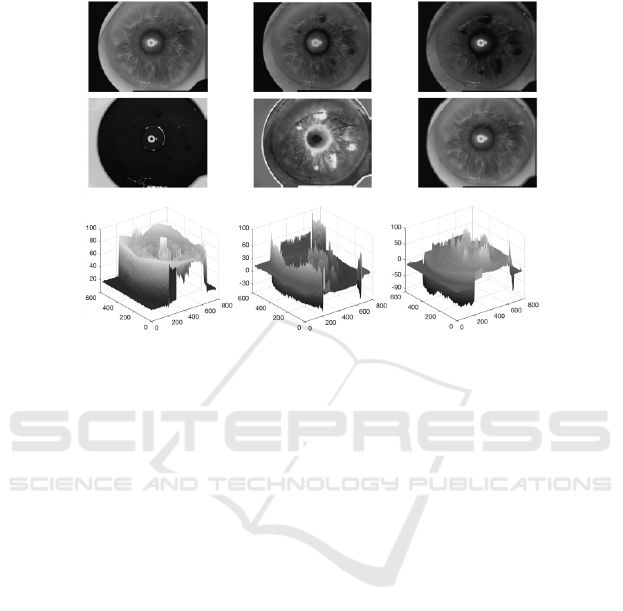
Figure 2: Color components of the image in Figure 1: upper panel (from left to right, R, G and B); middle panel (from left to

right, H, S and I); lower panel (from left to right, L∗, a∗ and b∗).

and blue light that has a speciﬁc color (Tkalcic and

Tasic, 2003). Thus, a color RGB image can be inter-

preted as a collection of three monochrome images,

one for each primary color. The upper panel in Fig-

ure 2 shows the R, G and B components associated

with the eye image displayed in Figure 1.

It is interesting to remark that the components in

the RGB color space present a high correlation be-

tween them, especially in natural images (Sangwine

and Horne, 2008).

2.2 HSI

Compared to the RGB model, the HSI model pro-

vides a more intuitive description of color for hu-

mans, describing color through three components;

hue (H), saturation (S) and brightness (I) (Gonz

alez

and Woods, 2007).

The HSI model, which decouples the intensity

component from the chromatic part (hue and satura-

tion), is deﬁned through a non-linear transformation

of the RGB color space. This transformation modi-

ﬁes the cube subspace of the RGB model, turning it

into two cones joined at their base. Geometrically,

the saturation component S corresponds to the radial

distance from the cone, quantifying the mixture with

white light. The component H describes the domi-

nant wavelength and is determined as the angle that

the particular color point makes with respect to the

angle of zero degrees (wavelength associated with a

red color). The range for H is [0, 360) degrees, with

an angular separation of 120 degrees between each

of the primary colors R, G and B. Lastly, the in-

tensity component I refers to the vertical axis of the

cones and incorporates achromatic information, with

low/high values of I corresponding to dark/light col-

ors. In general, both S and I take values in the interval

[0, 1], and H is usually normalized within [0, 1].

The middle panel in Figure 2 shows the H, S and I

components associated with the eye image displayed

in Figure 1.

2.3 CIELAB

The Commission Internationale d’Eclairage (CIE) is

a non-proﬁt organization devoted to publish standards

related to science, technology and art in the ﬁelds of

light and lighting. In 1976, the CIE proposed the

CIELAB space to deﬁne a perceptually linear repre-

sentation of color, characterized by representing the

separation between colors proportionally to the visual

differences between them.

The L ∗ a ∗ b∗ components are obtained by apply-

ing a set of nonlinear transformations to the RGB

model (Sangwine and Horne, 2008), providing a sub-

space that corresponds to a sphere. The component

L∗ represents the brightness of the color and contains

the achromatic information. The range of variation

of L∗ is the interval [0, 100]: values close to 0 rep-

resent dark colors up to black, while high values in-

SIGMAP 2022 - 19th International Conference on Signal Processing and Multimedia Applications

dicate light colors up to white. On the other hand,

the a∗ and b∗ components can take positive and neg-

ative values, and deﬁne a measure of the amount that

certain color is magenta-green and yellow-blue, re-

spectively. For a better visualization of the a∗ and

b∗ components (potentially with negative values), a

three-dimensional representation has been chosen in

the lower panel of Figure 2 (the xy plane corresponds

to the spatial coordinates of the image).

3 STATISTICAL APPROACHES

FOR QUANTIFYING IRIS

COLOR DIFFERENCES

There are not two identical irises, including those of

twins and even the two irises of one and the same per-

son (Juniati et al., 2020). However, we are not inter-

ested in the iris texture pattern structure, mostly de-

termined by ﬁbers, nerves and vessels. Instead, our

goal is to identify color differences in the eyes of the

same person, focusing on the global distribution of

the iris color. For this purpose, we consider the color

histograms (one histogram per color component) and

propose two techniques to quantify their differences.

3.1 Color Feature Vectors

The histogram of a monochrome image is a bar chart

representing the distribution of the pixel values in the

image (Gonz

alez and Woods, 2007). Each bar corre-

sponds to a group of values, determined by the width

of the bar (also named bin width), while the bar height

is the number of image pixels with values within the

bin. Regardless of the image size, values in the his-

togram are normalized to represent probability esti-

mations (calculated as relative frequencies).

Although the histogram discards information

about the spatial distribution of intensity levels, it is

a very useful tool in image analysis for image char-

acterization (Gonz

alez and Woods, 2007). Thus, his-

tograms allow the evaluation of image attributes such

as contrast and brightness. In general, a low con-

trast image will have the histogram bars clustered in

a narrow range, while an image with high contrast

will have a balanced histogram. In image process-

ing, histogram matching is used to transform the his-

togram of any image to a speciﬁc one. The histogram

equalization technique is a special case in which the

speciﬁed histogram is uniformly distributed. Though

we also consider histogram matching, our approach is

completely different, since no transformation is per-

formed, just a quantiﬁcation of the similarity between

histograms to determine their matching degree.

The basis of our work is inspired by the biometric

recognition system proposed in (Demirel and Anbar-

jafari, 2008), where each color component of the iris

image is characterized by a feature vector F obtained

from the corresponding histogram. The length of F

depends on the number of considered bins. In color

images, a histogram is represented for each compo-

nent of the color model. Color histograms in this work

are computed only considering the pixels associated

with the iris (manually segmented from the whole im-

age).

Let us assume L bins in the histogram, denoted

as b

, b

, ··· , b

L−1

and uniformly distributed in the

whole range of the corresponding color component.

Considering the RGB model, three feature vectors

, F

and F

representing the the color histograms

of the image I, are obtained:

= [ f

R,b

, ··· , f

R,b

L−1

]

= [ f

G,b

, ··· , f

G,b

L−1

]

= [ f

B,b

, ··· , f

B,b

L−1

]

(1)

To make the iris characterization independent on

the image and iris size, note that each feature vector

can be normalized so that its L elements can be inter-

preted as probabilities.

3.2 Cross Correlation

In the signal processing ﬁeld, cross-correlation allows

us to measure the similarity of two series as a function

of the displacement τ of one series relative to the an-

other one (Rabiner and Gold, 1975). Thus, the statis-

tical similarity between two images can be measured

by computing the cross-correlation between the his-

tograms of the respective images.

The authors of (Demirel and Anbarjafari, 2008)

propose to use the maximum absolute value of the

cross-correlation coefﬁcient between the color his-

tograms of a given iris and those associated with indi-

viduals in a database for iris recognition. The idea is

to determine the identity of the individual as the one

in the database for which the maximum value of the

cross-correlation coefﬁcient is obtained.

With a different approach, in this work we propose

to calculate the cross-correlation R between two fea-

ture vectors F obtained from histograms, see Eq.(1).

The feature vectors considered to compute R are as-

sociated with the same color component in each iris

(left and right, I

and I

) of the same individual I.

The mathematical formulation of cross-correlation is

dependent on the shift τ between sequences F

and

, as follows:

Statistical Analysis of Color Differences on Iris Images for Supporting Cluster Headache Diagnosis

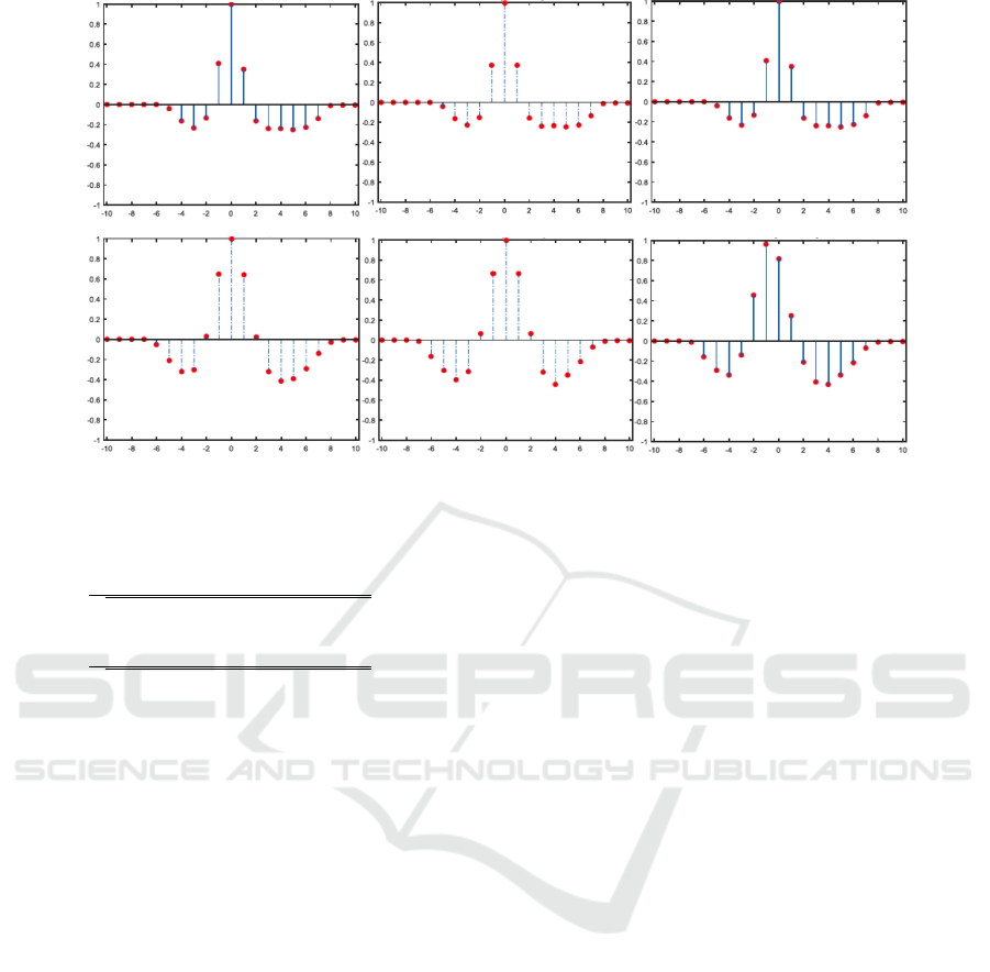
Figure 3: Average cross-correlation between feature vectors of the R component when considering the left iris (left panels),

the right iris (middle panels) and the left and right iris (right panels) of two patients: healthy patient (upper panels) and patient

with CH (lower panels).

R(τ) =











∑

L+τ−1

k=0

( f

k−τ

−

)( f

−

)

∑

L−1

k=0

( f

−

)

∑

L−1

k=0

( f

−

)

for τ < 0

∑

L−τ−1

k=0

( f

−

)( f

k+τ

−

)

∑

L−1

k=0

( f

−

)

∑

L−1

k=0

( f

−

)

for τ ≥ 0

(2)

where

and

are the average values of sequences

and F

, respectively. The denominator in Eq. (2)

has a normalization effect in the series R(τ), so that

the cross-correlation values are within [−1, 1]. Note

that R(τ) = 0 indicates no correlation, while maxi-

mum correlation is obtained for |R(τ)| = 1.

When considering a speciﬁc color component C,

our hypothesis is that the maximum correlation value

between F

and F

should be centered at τ=0 (no

shift). This would show a similar distribution for the

C-th color component in both eyes (bin rates coin-

cide with respect to their positions). Note that this

statement would be true as long as the comparisons

are made with identical bin widths and positions be-

tween the two histograms. Therefore, when calculat-

ing the maximum cross-correlation value between the

eye feature vectors of a healthy patient, values close

to one should be obtained at τ=0. This would show

that both sequences have the same structure regarding

the distribution of the intensity levels in a particular

color component. For the case of patients with CH,

it is expected that the maximum value is obtained for

τ 6= 0.

For illustration, Figure 3 shows the average cross-

correlation as a function of the shift τ between se-

quences. Feature vectors linked to the histogram of

the R component of the two irises of the same per-

son have been considered for two cases: a healthy pa-

tient (upper panels) and a patient diagnosed with CH

(lower panels). The average is computed over four

disjoint subsets of pixels in the same iris image, as de-

tailed in Subsection 4.1. Note that the highest cross-

correlation value corresponds to τ = 0 when the his-

tograms of the same iris (left or right) are considered,

both for the healthy and for the patient with CH. How-

ever, when considering cross-correlation between his-

tograms of the left and right irises, the highest cross-

correlation value is located in τ = 0 for the healthy pa-

tient and in τ = −1 for the patient with CH. This result

shows statistical differences in the distribution of the

intensity levels of the red color component in the left

and right irises for the patient with CH. Though only

results for the R component are presented, similar out-

comes are obtained when considering components G

and B for these cases.

3.3 Kullback-Leibler Divergence

In contrast to cross-correlation, which measures simi-

larity between two probability distributions linearly,

the Kullback-Leibler Divergence or D

(Kullback

and Leibler, 1951) provides a nonlinear measure of

the difference between two distributions.

Let be P and Q two probability distributions of

a discrete random variable with L possible values

in b

, ··· , b

L−1

, the Kullback-Leibler Divergence be-

tween P and Q is deﬁned by

SIGMAP 2022 - 19th International Conference on Signal Processing and Multimedia Applications

(P||Q) =

L−1

∑

i=0

P(b

)ln



P(b

)

Q(b

)



(3)

According to this measure, the closer the value of D

is to zero, the more similar P and Q are. In our sce-

nario, P and Q correspond to two feature vectors as

those in Eq. (1).

4 EXPERIMENTS AND RESULTS

4.1 Image Dataset

A set of 16 iris images from 8 patients obtained in the

Ophthalmology Department of the Hospital Univer-

sitario Fundaci

on Alcorc

on (Madrid, Spain) is avail-

able. The high-resolution camera Zeiss FF 450 plus

Fundus IE, 768x576 pixels with 451 Visupac Digi-

tal version 3.2.1 digital ﬁle system was used. Im-

ages were taken under the same light conditions and

exposure parameters, counteracting the effect of the

ﬂash by making the reﬂection on the pupil, trying

not to affect the iris brightness. The neurologist JA

Pareja-Grande performed the diagnosis of these pa-

tients, resulting in one healthy patient (HP), three pa-

tients who have some kind of pathology affecting the

iris color but it is not conﬁrmed that such pathology

is CH (DP1, DP2 and DP3), and four individuals with

conﬁrmed diagnosis of CH (CHP1, CHP2, CHP3 and

CHP4). Figure 4 and Figure 5 display the irises of

each patient in the study.

The iris segmentation is manually performed by

removing pupil and sclera. Subsequently, for a more

robust statistical analysis, the pixels of each iris are

separated into four disjoint subsets or patitions. Pix-

els for each partition were randomly distributed in

the iris, so that the values of cross-correlation and

Kullback-Leibler divergence presented in the follow-

ing tables are averaged.

4.2 Use of Histogram Cross-correlation

The average cross-correlation was computed consid-

ering each component of the three color subspaces.

Following the approach presented in Subsection 3.2,

just the healthy patient (HP) was correctly identiﬁed

by using the cross-correlation of each of the nine

color components. For patients identiﬁed as CHP2,

CHP3 and CHP4, the cross-correlation technique did

not identify color differences in any component of the

three color spaces. For the group of patients with no

conﬁrmed CH diagnosis, cross-correlation of at least

one component of each color space revealed differ-

ences between both irises for two of the three patients

(DP1 and DP2) in Figure 4.

After analyzing these results, we concluded that

the histogram cross-correlation does not seem ade-

quate to identify most of the patients with CH in our

dataset. In fact, just the patient with the most evident

differences in the iris color (CHP1) is identiﬁed.

4.3 Use of Kullback-Leibler Divergence

We present now in Table 1 the average values of D

computed when considering the same color feature

vectors as those in Subsection 4.2. Each row in Table

1 is associated with a color component, and each col-

umn refers to the D

when considering probability

distributions (computed from Eq. (1)) within the same

eye and between both eyes of the same patient. Note

that the obtained values do not seem comparable be-

tween patients: for example, the D

for the compo-

nent H when considering both irises of the healthy pa-

tient takes the value 0.01731, which is higher than that

associated with the component H of CHP1 (0.00384),

which in principle is contrary to our hypothesis (diver-

gence value closer to 0, more similar distributions).

Since there can also be signiﬁcant differences

in absolute values when comparing estimates of the

mass probability function (obtained from the iris par-

titions) in the same iris, we propose to compute a rel-

ative measure. It is obtained by normalizing the D

when considering feature vectors of both irises with

the D

obtained using feature vectors of each of the

irises. The results are shown in Table 2 and Table 3,

i.e. two tables to consider all patients in our dataset.

As an example, the value 27.16 in the ﬁrst column and

ﬁrst row in Table 2 is obtained as the ratio between

0.00718 and 0.00026.

From Table 2, none of the D

ratios exceeds two

orders of magnitude for the case of the healthy patient

(column HP). In contrast, for all patients with CH (Ta-

ble 3) there is always at least one component of the

three color spaces for which this ratio exceeds 100

(two orders of magnitude). For example, in the case of

CHP1, the RGB color space seems to be the most suit-

able for identifying differences between irises, with

high difference in the relative distributions between

irises for the the three components. The L ∗ a ∗ b∗

space seems best suited to show differences in the

case of CHP2, while only the component b∗ shows

a ratio greater than 100 (shown in bold). For CHP4,

the components H and S seem the least appropriate

for showing color differences in the irises. Again,

these two components offer the least relative differ-

ence for the patient DP3. It is interesting to remark

that, in general, patients with CH do not show in our

Statistical Analysis of Color Differences on Iris Images for Supporting Cluster Headache Diagnosis

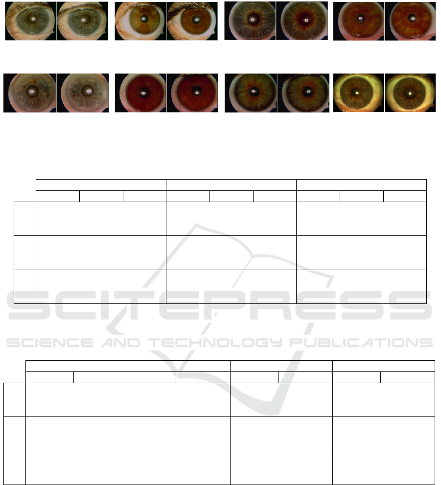
Figure 4: Left and right iris images associated with: the healthy patient (left, identiﬁed as HP) and three patients with doubt

in the CH diagnosis (patients identiﬁed from right to left as DP3, DP2 and DP1).

Figure 5: Left and right iris images associated with patients diagnosed with CH, named: CHP1 (left), CHP2, CHP3 and CHP4

(right).

Table 1: Average D

for each component of the RGB, HSI and L ∗ a ∗b∗ spaces when three patients are considered: HP, DP1

and CHP1. For each patient, only the left iris (column labeled “Left”), only the right iris (column labeled “Right”) and both

irises (column labeled “Both”) are considered.

HP DP1 CHP1

Left Right Both Left Right Both Left Right Both

R 0.00026 0.00059 0.00718 0.00086 0.00049 0.69376 0.00023 0.00024 0.20515

G 0.00036 0.00054 0.02151 0.00060 0.00067 1.58974 0.00014 0.00019 0.23238

B 0.00026 0.00059 0.02301 0.00039 0.00041 0.75488 0.00016 0.00019 0.26849

H 0.00109 0.00075 0.01731 0.00081 0.00056 0.13888 0.00044 0.00046 0.00384

S 0.00075 0.00084 0.05878 0.00061 0.00088 0.59718 0.00036 0.00047 0.19486

I 0.00084 0.00070 0.02580 0.00076 0.00071 1.24638 0.00042 0.00056 0.26411

L∗ 0.00024 0.00029 0.01895 0.00026 0.00032 1.15035 0.00022 0.00018 0.22983

a∗ 0.00011 0.00006 0.00172 0.00010 0.00004 0.61492 0.00001 0.00002 0.00102

b∗ 0.00010 0.00019 0.00281 0.00010 0.00006 0.04871 0.00006 0.00003 0.00558

Table 2: Ratio of the average D

for each component of the RGB, HSI and L∗a∗b∗ spaces when four patients are considered:

HP, DP1, DP2 and DP3. For each patient and color component, the column labeled “Both/Left” contains the ratio of the

average D

of both irises to that of the left irises, while column labeled “Both/Right” refers to the ratio of the average D

of both irises to that of the right iris. Figures in bold indicate relative measures greater than 100.

HP DP1 DP2 DP3

Both/Left Both/Right Both/Left Both/Right Both/Left Both/Right Both/Left Both/Right

R 27.61 12.17 806.69 1415.83 270.32 273.66 1489.91 927.85

G 59.75 39.83 2649.57 2372.74 702.74 654.72 139.67 109.66

B 88.50 39.00 1935.59 1841.17 3027.95 2813.13 145.57 91.48

H 15.88 23.08 171.45 248.00 287.84 251.08 29.26 21.88

S 78.37 69.98 978.98 678.61 1858.27 1797.27 21.73 22.11

I 30.71 36.85 1639.97 1755.46 516.85 561.16 351.85 169.85

L∗ 78.95 65.34 4424.42 3594.84 604.06 667.40 616.42 416.77

a∗ 15.63 28.67 6149.20 15373.00 2779.63 2150.27 1577.93 1110.57

b∗ 28.10 14.78 487.10 811.83 3203.30 14092.98 2024.80 1589.49

(reduced) dataset the highest relative differences.

From the results, it could be concluded that inter-

mediate values of the proposed relative measure lead

to a clearer diagnosis of CH, while more pronounced

color differences (see results for DP1 and DP2) might

not be so closely related to the same stages of CH di-

agnosis, or even be related to other pathologies.

5 CONCLUSIONS AND FUTURE

WORK

In this work, we have addressed the suitability of the

cross-correlation series compared with the Kullback-

Leibler divergence in order to provide us with qual-

ity biomarkers for cluster headache. Whereas pre-

vious efforts had been devoted to design machine

learning schemes accounting for the differences in

SIGMAP 2022 - 19th International Conference on Signal Processing and Multimedia Applications

Table 3: Ratio of the average D

for each component of the RGB, HSI and L ∗ a ∗b∗ spaces when the four patients diagnosed

with CH are considered. For each patient and color component, the column labeled “Both/Left” contains the ratio of the

average D

of both irises to that of the left irises, while column labeled “Both/Right” refers to the ratio of the average D

of both irises to that of the right iris. Figures in bold indicate relative measures greater than 100.

CHP1 CHP2 CHP3 CHP4

Both/Left Both/Right Both/Left Both/Right Both/Left Both/Right Both/Left Both/Right

R 891.95 854.79 384.47 355.80 20.01 21.03 575.23 306.46

G 1659.85 1223.05 235.53 115.95 24.80 21.25 1178.46 768.58

B 1678.06 1413.10 78.81 54.22 52.96 16.93 221.62 179.19

H 8.72 8.34 1351.64 267.01 29.01 28.05 28.18 43.88

S 541.27 414.59 136.11 98.56 20.50 18.61 83.89 96.73

I 628.83 471.62 545.83 525.34 17.53 23.45 654.68 418.55

L∗ 1044.68 1276.83 1135.23 401.34 17.36 35.80 1370.98 999.81

a∗ 102.00 51.00 692.14 454.07 8.43 12.84 135.49 196.85

b∗ 93.00 186.00 1048.50 518.60 135.27 222.59 984.58 1059.58

color of a given patient with direct representation of

color neighborhood of each pixel, here we focused on

building principled features based on color space his-

tograms.

Our results show that the difference between iris

coloration can be detected in terms of both luminance

and chrominance, as the color resulting from melanin

concentration is also dependent of brightness. In ad-

dition, cross-correlation based schemes seem to ex-

hibit low detection capabilities, whereas the relative

measure based on the Kullback-Leibler Divergence

seems to provide us with good results. That is, the

proposed procedure based on D

provides moder-

ate ﬂuctuations in healthy subjects, yielding increased

ﬂuctuations in some (or even all) components of the

color spaces in the case of patients with CH.

The most evident limitation of our study is the re-

duced number of iris images, which also include pa-

tients with doubted diagnostic of CH. It is interesting

to remark that assembling this kind of images repre-

sents an additional workload for clinicians and hospi-

tal staff. In this sense, the present work evidences that

digital signal processing could provide us with suit-

able biomarkers for CH diagnosis and their use in the

clinical environment.

ACKNOWLEDGEMENTS

This work has been partly supported by the Spanish

Research Project PID2019-106623RB-C41.

REFERENCES

Demirel, H. and Anbarjafari, G. (2008). Iris recogni-

tion system using combined histogram statistics. In

Proceedings of the 23rd International Symposium on

Computer and Information. IEEE.

El-Yaagoubi, M., Mora-Jim

enez, I., Jabrane, Y., Mu

noz-

Romero, S., Rojo-

Alvarez, J., and Pareja-Grande, J.

(2020). Quantitative cluster headace analysis for neu-

rological diagnosis support using statitical classiﬁca-

tion. Information, 11(393):1–13.

Gonz

alez, R. and Woods, R. (2007). Digital Image Process-

ing. Pearson Prentice Hall, 3rd edition.

Juniati, D., Budayasa, I., and Khotimah, C. (2020). The

similarity of iris between twins and its effect on iris

recognition using box counting. Communications in

Mathematical Biology and Neuroscience, (90):1–13.

Kullback, S. and Leibler, R. (1951). On information

and sufﬁciency. Annals of Mathematical Statistics,

22(1):79–86.

Ma, L., Tan, T., Wang, Y., and Zhang, D. (2003). Personal

identiﬁcation based on iris texture analysis. IEEE

Trans Pat An Mach Intel, 25:1519–33.

Pareja, J., Espejo, M., Trigo, M., and Sjaastad, O.

(1997). Congenital horners syndrome and ipsilateral

headache. Funct. Neurol., 12:123–31.

Rabiner, L. and Gold, B. (1975). Theory and Application of

Digital Signal Processing. Prentice Hall.

Sangwine, S. and Horne, R. (2008). The Colour Image Pro-

cessing Handbook, chapter 4, pages 67–90. Chapman

and Hall.

Tkalcic, M. and Tasic, J. (2003). Colour spaces: Perceptual,

historical and applicational background. In The Re-

gion 8 EUROCON 2003. Computer as a Tool. IEEE.

Wielgus, A. and Sarna, T. (2005). Melanin in human irides

of different color and age of donors. Pigment Cell

Res., 18:454–64.

Statistical Analysis of Color Differences on Iris Images for Supporting Cluster Headache Diagnosis