
Spline Modeling and Level of Detail for Audio
Matt Klassen
DigiPen Institute of Technology, Willows Road, Redmond, WA, U.S.A.
Keywords:
Spline, Audio, Signal, Interpolation, Cycle, Level, Detail.
Abstract:
In this paper we propose spline models of audio as the first step toward a hierarchical system of level of
detail (LOD) for audio rendering. We describe methods such as cycle interpolation which can produce spline
models and approximations of audio data. These models can be used to render output in realtime, but can
also be mixed prior to rendering. Examples of audio data simplified to spline models with cycle interpolation
can reduce the data to less than 2% of the full resolution data size, with only minor impact to audio quality.
We present a sequence of such examples with instrument models. We also introduce the idea of pre-rendered
filtering and mixing, based on the B-spline coefficients of the models.
1 INTRODUCTION
Level of Detail (LOD) for graphics has played an im-
portant role in realtime rendering for the past forty
years, beginning with flight simulators in the 1980’s
and culminating in the realtime video game engines of
today (see (Luebke, 2003) section 1.2 History). LOD
can be thought of as a collection of cost-saving meth-
ods, in both memory and computation, based on a
hierarchical approach. A naive example carries the
main idea: A car is in moving in the distance on a
video screen. The viewer cannot perceive any sig-
nificant detail, and neither would they in the real life
experience that the scene is imitating. It is suffi-
cient to represent the car with a very simple low poly-
gon model. This saves in not having to load a com-
plex model into memory, and not having to render
the many vertices and textures of a complex model
through the graphics pipeline. We will refer to this
type of model as a low resolution model. There are
many more aspects to consider, but first consider the
analogous question for audio: If the car is also mak-
ing some engine sounds, what is the equivalent low
resolution audio model of this sound?
In order to make the question a bit more precise
we ask: What should a low resolution audio model
consist of, and what should be required of a low res-
olution model? First, it should consist of model data
which has a smaller footprint than the final full res-
olution audio stream. Second, an approximation of
the full resolution version should be computable lo-
cally from the model data. Third, this approximation
should be usable as a distant sound, much in the same
way that the low polygon object is usable visually.
Fourth, a low resolution audio model should be mix-
able with other sounds at the same level of detail using
the model data prior to rendering.
It is also important to note what we do not mean
by a low resolution model. First, we do not mean a
compressed audio format. Typical compression al-
gorithms do a marvelous job of conserving storage
space, but in order to use a compressed file it must first
be decompressed. This means that we cannot com-
pute output values locally from the model data, nor
can we mix audio files in compressed format. By low
resolution model we also do not mean a purely com-
putational model, or what is often called a physical
model. In the best cases, such models may be the ul-
timate replacement for static audio files, but they can
also take considerable effort to build, maintain and
use, and are in a different class by themselves.
We propose that spline models of audio signals
can satisfy the basic requirements for low resolution
audio models and become the first step in hierarchical
level of detail for audio. The basic models and cycle
interpolation are introduced in (Klassen, 2022). In
this paper we introduce a more flexible variant of the
basic model, the delta model, which adapts better to
cycle interpolation and in some cases solves the shape
discontinuity problem from (Klassen, 2022). We also
discuss methods for rendering, mixing, and error cal-
culations.
Since LOD is well established for graphics, we
also continue the analogy between graphics and au-
94
Klassen, M.
Spline Modeling and Level of Detail for Audio.
DOI: 10.5220/0011321500003289
In Proceedings of the 19th International Conference on Signal Processing and Multimedia Applications (SIGMAP 2022), pages 94-101
ISBN: 978-989-758-591-3; ISSN: 2184-9471
Copyright
c
2022 by SCITEPRESS – Science and Technology Publications, Lda. All rights reserved

dio. For instance, a high resolution graphics model
may have many vertices, and one way to simplify such
models is to remove vertices but still preserve some
of the geometry. In the case of audio, we can think
of the cycle as playing the role of a vertex. An inter-
esting audio signal, such as a single note played on a
piano or guitar, has many cycles evolving over time
at some approximate fundamental frequency f
0
. It is
possible with spline modeling and cycle interpolation
to remove many cycles but replace them with interpo-
lated versions when rendering, thus arriving at lower
resolution models.
What problem does LOD for audio solve? In mod-
ern realtime multimedia applications, such as video
games and virtual reality, the demands on computa-
tion and memory continue to rise rapidly. This can
also be compounded by the number of simultaneous
sound sources being used. A common solution is to
use submixes, so that the number of voices (or audio
streams) in play at any time can be limited by group-
ing together voices which share common character-
istics. Higher priority voices, such as those in the
foreground and which are critical to a given scene,
are given more attention. For instance, it may be
that a single key character emits sounds of different
types, say vocalizations, weapon sounds, footsteps,
each with its own audio stream. Each of these sounds
may also have effects ranging from simple filters to
HRTF for spatial localization. The cost of such high
priority detail must be offset by the savings in treating
low priority sounds more economically. If many low
priority sounds are dynamically being grouped into a
particular submix, say a distant group of characters
or objects, it may be significant to work with lower
resolution sounds which can also be mixed prior to
rendering.
2 SPLINE MODELS
The basic spline model is discussed in (Klassen,
2022), which we summarize here. The main enhance-
ment to this model, which we introduce in this pa-
per, is that we allow cycles to be defined without
the requirement that they begin and end with zero-
crossings. We refer to this modified model as the delta
model, since it amounts to introducing a small vertical
shift to the ends of each cycle. This shift is inserted in
the form of a cubic polynomial which can be thought
of as replacing the time axis over the interval of one
cycle. This delta model arose initially to solve the
“shape discontinuity” problem described in (Klassen,
2022).
As a basic class of sounds or signals, we use in-
strument samples with known fundamental frequency.
This allows us to work with the notion of a cycle, or
period, as a basic signal block. Although this is not
well-defined, given that the length and shape of cycle
can both vary with time, it is often how sound presents
itself, and is quite compelling. (We also note that
these methods can be adapted to work with arbitrary
fixed size audio blocks, but that the methods of cy-
cle interpolation are more clearly demonstrated when
there is an approximate notion of cycle available.) For
example, if we consider a simple recorded sound such
as a single note played on a piano or a guitar, the sig-
nal can be partitioned approximately into cycles based
on zero-crossings. This approach is central to the ba-
sic model in (Klassen, 2022). In the basic model, once
the cycles are determined by the sequence of zeros
z
i
, i = 0, ..., p, we do a cubic B-spline fit to the au-
dio sample data. We assume the audio sample data is
given as a piecewise linear function of time t, mean-
ing that we can choose to interpolate between samples
linearly for the purpose of defining zero-crossings. To
specify the spline function, say f (t), we work with
a uniform sequence of k subintervals on the interval
[0,1], and the vector space of C
2
cubic polynomial
splines with dimension n = k + 3. To specify a basis,
we use the knot sequence:
t = {t
0
,... ,t
N
} = {0,0,0,0,
1
k
,
2
k
,... ,
k − 1
k
,1,1,1, 1}.
Writing the B-spline basis functions associated to t as
B
0
(t),B
1
(t),.. . ,B
n−1
(t)
we note that B
0
(0) = 1 and B
n−1
(1) = 1, and all the
other basis splines vanish at both 0 and 1. So we
set c
0
= c
n−1
= 0 and solve for the other n − 2 co-
efficients for each cycle. In order to approximate the
audio data in one cycle, we find an interpolating cu-
bic spline which matches the (piecewise linear) audio
data function x(t) at n − 2 = k + 1 specified points. A
simple choice of such points is to use k−1 subinterval
endpoints and then add two more points at the middle
of the first and last subintervals.
In Figure 1 is a portion of the graph of an au-
dio sample, cycles 10 through 15 of a guitar pluck
at approximately 450 Hz, with spline model in blue.
Here we are using the default d = 3, interpolating cu-
bic spline on each cycle, with k = 15 subintervals
hence dimension n = 18. This signal is recorded
at 44100 samples per second, so there are around
98 = 44100/450 samples per cycle. The actual num-
ber of samples per cycle is listed at the bottom of each
shaded cycle. Since we are using only 18 data points
to define the interpolating spline, the match to the au-
dio graph is clearly not exact. For this audio sample,
if we use k = 30 and n = 33, the spline graph is diffi-
cult to distinguish from the original.
Spline Modeling and Level of Detail for Audio
95

Figure 1: Spline model of guitar pluck.
Next, we add the changes for the delta model,
the values y
0
and y
1
. It is important to note that to
solve for the spline function f in the delta model, we
use as interpolation targets the difference x(t) − p(t),
with p(t) = y
0
+ δq(t), where q(t) = 3t
2
− 2t
3
, and
δ = y
1
− y
0
. We summarize the data per cycle, before
explaining how the choice of y
0
and y
1
can be made
in constructing the delta model.
Data per cycle for the delta model:
• degree d = 3
• number of subintervals k
• subinterval sequence: [u
i
,u
i+1
] = [
i
k
,
i+1
k
],
i = 0, ..., k − 1
• endpoint values y
0
and y
1
• cubic polynomial p(t) = y
0
+ δq(t), δ = y
1
− y
0
• knot sequence: t = {t
0
,... ,t
N
}
= {0,0,0,0,
1
k
,
2
k
,... ,
k−1
k
,1,1,1, 1}
• dimension of the vector space V of B-spline
functions: n = k + 3 = N − 3
• B-spline basis functions: B
0
(t),.. . ,B
n−1
(t)
• interpolating spline with c
0
= c
n−1
= 0:
f (t) = c
1
B
1
(t) + · ·· + c
n−2
B
n−2
(t)
• input values: s
0
= 0,s
1
=
1
2k
, s
i
= u
i−1
,
i = 2, ..., n − 2, s
n−2
= 1 −
1
2k
,s
n−1
= 1
• target values: x(s
0
) − p(s
0
), x(s
1
) − p(s
1
),...,
x(s
n−1
) − p(s
n−1
)
Now we can define the delta model to be the se-
quence of cycle endpoints (formerly zero-crossings)
z
j
, j = 0, . ..,N, with the accompanying y-values y
j
=
x(z
j
), and the sequence of spline functions f
j
(t) on
the intervals [z
j
,z
j+1
]. We also refer to each of these
splines and their associated data as one “cycle” C
j
, so
that the delta model is the sequence of cycles C
j
for
j = 0,..., N − 1. Further, let the B-spline coefficients
for cycle C
j
be c
j
i
, i = 0, . ..,n − 1. For the purpose
of analysis we keep the B-spline coefficients separate
from the values of the cubic polynomial p(t), but for
rendering purposes these can be easily combined into
one set of B-spline coefficients by way of the polar
form for q(t). In particular, the B-spline coefficients
for q(t) are computed from its polar form
F[x, y,z] = xy + xz + yz − 2xyz
and knot sequence t as
c
i
= F[t
i+1
,t
i+2
,t
i+3
], i = 0, ..., n − 1.
Next we describe how the determination of cycle
endpoints z
j
and values y
j
can be made through an
optimization process. The goal is to choose endpoints
for a cycle based on similarity to the previous cycle
shape. In particular, suppose that an initial cycle or
sequence of cycles is chosen based on zero-crossings.
Then we would like to choose cycles going forward
in such a way as to maintain the shape of the curve
from cycle to cycle. This can be achieved through
the measurement of error between successive cycles.
For example, we will define a weighted error on the
choice of right endpoint of C
j
to be computed as fol-
lows: First, project the right endpoint for cycle j in
the usual way as in the basic model, by simply let-
ting z
j+1
= z
j
+ P
0
where P
0
is the period length pre-
dicted by the fundamental frequency f
0
. Next, define
a spline function f
j
(t) for C
j
by using the B-spline co-
efficients from cycle j − 1 with the endpoints of cycle
SIGMAP 2022 - 19th International Conference on Signal Processing and Multimedia Applications
96

j. Since we work on [0,1], this means to use the y-
values from the endpoints of C
j
determined from the
signal values there: y
0
= x(z
j
) and y
1
= x(z
j+1
). Next,
compute sample output values on C
j
with this spline
model f
j
, and compare to the actual audio sample
data. Call the mean-square difference in these sample
values E
0
j
. Then do the same for the derivative f
0
(t)
and an approximate or discrete derivative for x(t) and
call the mean-square difference in these values E
1
j
.
Define the error for the choice of z
j+1
= z
j
+ P
0
to
be
E
j
(0) = α
0
E
0
j
+ α
1
E
1
j
for some choice of weights α
0
+ α
1
= 1. In practice
we have found that the values α
0
= 0 and α
1
= 1 al-
ready work quite well in order to solve the shape dis-
continuity problem. Next, we choose a small value
ε > 0 and compute the same error but now for choices
z
j+1
= z
j
+P
0
±rε, for integers r < L, for some bound
L. For these integers r define
E
j
(r) = α
0
E
0
j
(r) + α
1
E
1
j
(r).
Finally, choose the value of r that minimizes E
j
(r)
and set the cycle C
j
using this z
j+1
.
One interesting observation with this error mini-
mization is that the cycles in a model can drift. By
this we mean that the error tolerance allows for the
endpoints to shift gradually to the right of the per-
ceived cycle shape when viewed over many cycles.
This can be resolved by putting another term in the
error which is a penalty for increasing value y
1
, for
instance α
2
y
2
1
to obtain:
E
j
(r) = α
0
E
0
j
(r) + α
1
E
1
j
(r) + α
2
y
2
1
(r).
This approach tends to maintain cycle shape more
consistently, allowing for effective cycle interpola-
tion, especially in the case of shape discontinuities
induced by cycles defined using zero-crossings.
We refer here to the reference example in
(Klassen, 2022) and the shape discontinuity which oc-
curs at cycle number 181. If we use the delta model
as described above, with bound L = 10 samples, and
k = m = 20, the cycle interpolation works well and
the model uses about 1.5% of the full resolution data.
3 INSTRUMENT MODELS
We describe here a sequence of instrument models
for a one second audio sample with fundamental fre-
quency f
0
somewhere in the octave starting at mid-
dle C, or 261.6 Hz. These models are computed with
our Audio Spline Modeling software written in C++
with JUCE. Each instrument model is computed from
Figure 2: Spectrum of french horn sample.
a short audio sample, with bit depth 16 and sample
rate 44100 Hz, of at least one second in length. The
first step is to compute the delta model with frequency
guess f
0
and k = 30 subintervals. The dimension
of the resulting vector space of cubic splines is then
n = k + 3 = 33. We choose to use the following key
cycle indices, biased towards the attack phase at the
start of the sample:
0,5,10,15, 20, 25,30,40,50, 60, 70,80,
100,120,150,180, 220, f
0
.
With these 18 key cycles we use cycle interpolation
(with linear meta-splines) to construct the intermedi-
ate cycles. Additionally we use a linear ramp down
over the last 2/3 of one second. In these models the
data stored, as B-spline coefficients, for the 18 key cy-
cles is 18 · 33 = 594 values. As a percent of the total
number of values at full resolution, this is 594/44100
or about 1.35%.
To see how closely these models can match the
original waveforms, we illustrate this process with a
french horn sample with f
0
= 315 (E[ above middle
C). In Figures 2 and 3 are graphs of the spectrum
for the french horn sample (with ramp down applied,
for consistency) and the model as described above,
graphed with Audacity software. The FFT size used
is 1024 samples, and the Hann window is used to im-
prove frequency resolution.
In Table 1 we give the magnitude of the first ten
harmonic frequencies in decibels. These values are
obtained from the spectrum plots and are indicated
in dB, with 0 as full scale or maximum possible sig-
nal value. Note that the harmonic frequencies, which
are maximum points on the spectrum graphs, are not
strictly harmonic partials since they are not integer
multiples of the fundamental f
0
.
We compute two quantities to summarize this ta-
ble: First, the average ∆(dB)
avg
of the absolute differ-
Spline Modeling and Level of Detail for Audio
97
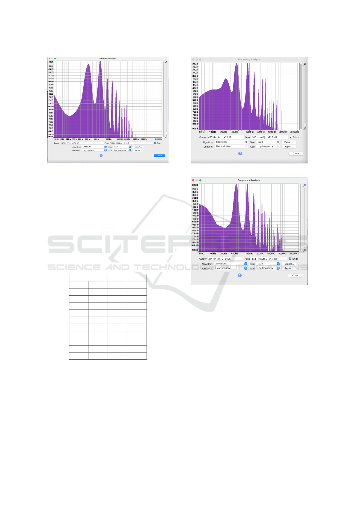
Figure 3: Spectrum of french horn model.
ence in the decibel values at each of the frequencies,
and second, the average ¢
avg
of the absolute cent val-
ues for the frequency ratio of the original and model
harmonic frequencies. Note, the cent value measure-
ment of the interval between two frequencies is de-
fined as:
¢(F
1
,F
2
) =
1200
log(2)
log
F
2
F
1
.
For this french horn model we find that
∆(dB)
avg
= 0.98 and ¢
avg
= 4.51.
Table 1: French horn harmonic amplitudes.
original model
Hz dB Hz dB
315 -19.0 315 -19.1
624 -14.5 624 -14.5
935 -32.2 939 -32.8
1253 -35.2 1259 -34.9
1563 -41.9 1566 -42.1
1873 -53.9 1875 -53.0
2181 -53.6 2192 -55.9
2494 -56.7 2508 -58.9
2811 -57.2 2816 -58.0
3121 -62.7 3126 -65.1
Next we present the same for a guitar pluck sam-
ple and model. The guitar pluck has fundamental
frequency approximately 445 Hz and is recorded at
sample rate 44100 Hz. Note the prominent subhar-
monic in the sample spectrum, at around 220 Hz. This
can already be seen in the pattern of cycles in Fig-
ure 1 where cycles 10 and 11 together form a cycle
which appears to be repeated in cycles 12 and 13. In
fact, we can model this waveform by selecting the fre-
quency guess 220, which restores the subharmonic in
Figure 4: Spectrum of guitar pluck sample.
Figure 5: Spectrum of guitar pluck model.
the model. In that case, as pointed out in (Klassen,
2022), there will be a new subharmonic at around 110
Hz. It is expected that a model which uses cycle in-
terpolation will not preserve submarmonics below the
fundamental frequency, since any oscillatory pattern
between two key cycles, say 100 and 120, will be lost
in the smooth interpolation as cycle 100 evolves into
cycle 120. However, it is shown in (Klassen, 2022)
that the subharmonic with 110 Hz can be simulated
by an alternating pattern of parabolas.
For this guitar pluck model we find that
∆(dB)
avg
= 1.12 and ¢
avg
= 5.41.
Finally, we give one more example for a flute sam-
ple and model in Table 3, and we collect the average
errors for comparison in Table 4.
SIGMAP 2022 - 19th International Conference on Signal Processing and Multimedia Applications
98

Table 2: Guitar pluck harmonic amplitudes.
original model
Hz dB Hz dB
445 -22.7 444 -21.8
883 -21.4 882 -21.3
1328 -31.5 1321 -30.8
1774 -47.7 1764 -47.4
2213 -38.5 2207 -38
2654 -38.2 2648 -37.8
3084 -66.6 3083 -61.8
3548 -54.9 3535 -55.2
3988 -47.1 3978 -48.3
4439 -58.6 4415 -60.6
Table 3: Flute harmonic amplitudes.
original model
Hz dB Hz dB
448 -11.4 447 -11.5
892 -27.8 889 -28.0
1343 -33.0 1344 -33.0
1786 -31.7 1783 -31.8
2227 -47.9 2225 -49.6
2679 -51.4 2675 -51.9
3123 -66.8 3118 -67.1
3560 -72.1 3560 -71.6
4016 -76.7 4010 -77.3
4445 -80.4 4456 -74.9
4 MODEL SIMPLIFICATION
In LOD for graphics there are many ways to do Mesh
Simplification (see chapter 2 of (Luebke, 2003)). For
audio, model simplification, or data reduction, can be
achieved in at least two different ways: 1) cycle in-
terpolation (compared to vertex removal), and 2) In-
terpolation point removal, which is a finer version of
1). The primary motivation for interpolation point re-
moval within one cycle is the existence of portions of
the cycle which have very small deviation in curva-
ture. The lower such deviation is, the more suitable
it can be to represent such a portion with one cubic
curve, meaning that it is possible to consider remov-
ing many interior knots on the interval defining that
portion of the cycle. Adaptive algorithms for refin-
ing knot sequences of splines have been used in (Park
and Lee, 2007) for B-spline curves in graphics. Sim-
ilar algorithms can be used for the B-spline functions
representing one audio cycle. This can lead to large
savings in amount of data in the model, but at the cost
of regularity.
Table 4: Model average errors for three instruments.
instrument ∆(dB)
avg
¢
avg
french horn 0.98 5.06
guitar 1.12 5.41
flute 0.95 2.77
5 ERROR MEASUREMENTS
When comparing lower resolution models to full res-
olution, whether for graphics or audio, the goal is to
achieve reasonable quality appropriate to the place-
ment of, or role played by, the rendered version in the
final scene, or mix. We have indicated how error func-
tions can be useful in computing the cycle endpoints
in the delta model. This achieves some accuracy when
removing cycles with cycle interpolation, since the er-
ror minimization is designed to give minimal changes
to B-spline coefficients from one cycle to the next.
Another approach is make global error measure-
ments for the rendered approximation from the model
in the frequency domain. One such error is the
relative amplitude spectral error used by Horner in
(Horner, 2013) to compare spectral qualities of musi-
cal sounds to resynthesized versions of those sounds
using FM and wavetable synthesis. It is useful to
assume an approximate fundamental frequency f
0
,
and to compute time-varying j
th
harmonic amplitudes
b
j
(t) of the full resolution sound, and b
0
j
(t) of the low
resolution sound, for various t. Suppose that these
time values are τ
i
and that the number of audio frames
(or samples) is N
f
, and the number of harmonic am-
plitudes to compute is N
h
. Then the error is defined
as:
ε =
1
N
f
N
f
∑
i=1
"
∑
N
h
j=1
(b
j
(τ
i
) − b
0
j
(τ
i
))
2
∑
N
h
j=1
b
j
(τ
i
)
2
#
1/2
6 PRE-RENDERED FILTERING
First we make a few observations on the knot se-
quence we are using for basis B-splines on each cycle.
Since we use 4 equal knots at the beginning and end,
and otherwise regularly spaced knots, then all cubic
B-splines defined by sequences of 5 consecutive knots
are translates of the same C
2
basis spline, except for
the first three B
3
0
(t), B
3
1
(t), and B
3
2
(t), and the last
three B
3
n−3
(t), B
3
n−2
(t), and B
3
n−1
(t). This leads to
some simple observations regarding delaying and fil-
tering of B-spline coefficients. Some of these filtering
methods also coincide with the methods of cellular
automata applied to B-spline coefficients of cycles, as
Spline Modeling and Level of Detail for Audio
99

in (Klassen and Lanthier, 2022).
For example, suppose that there are ρ samples per
subinterval, so ρ samples in any interval of length L
between knot values, and suppose t is in the inter-
val [t
J
,t
J+1
). Then to compute the spline value f (t),
by the de Boor algorithm, we use only the coeffi-
cients c
J−3
, c
J−2
, c
J−1
and c
J
. Similarly, to compute
f (t − L) we use the coefficients c
J−4
, c
J−3
, c
J−2
and
c
J−1
. So if we apply a delay operator to these coeffi-
cients, shifting by one index left, then we are comput-
ing values of f by a delay of 5 samples. This is true
as long as the B-splines used to compute values in the
interval [t
J−1
,t
J
) are exact shifts of those in [t
J
,t
J+1
),
which holds if 3 ≤ J < n − 3, or equivalently that the
value t is at least 3/k distance from the cycle end-
points. So the delay by one B-spline coefficient can
be locally viewed as a delay by ρ samples, within one
cycle, with the added restriction that we stay away
from the endpoints.
Now suppose that we apply the filter equation to
B-spline coefficients, with inputs c
i
c
0
i
=
1
2
(c
i
+ c
i−1
),
and outputs c
0
i
. This looks like a low-pass filter, but
when the result is used to compute samples, it has the
effect
y
t
=
1
2
(x
t
+ x
t−ρ
)
which is an inverse comb filter, but applied only to the
middle portion of cycles.
7 PRE-RENDERED MIXING
Since B-spline models contain data which can be used
to render the model to samples, locally in time, one
can ask if it is possible mix these models prior to ren-
dering. Since the goal of LOD is often efficiency, the
idea of mixing prior to rendering could be an advan-
tage. For example, if there are many voices which
need to be dynamically mixed at a low level of de-
tail, it will take much more memory and computa-
tion to render each voice and add the samples, than it
will to merge the data for each model and then ren-
der one voice, the mix. Under certain circumstances
it is straight-forward to do this type of pre-rendered
mixing. For example, if two cycles are defined for
the same time interval, say [a,b], and have the same k
value and B-spline basis, then mixing these two sig-
nals can be accomplished by simply averaging the two
sets of B-spline coefficients, since the result is no dif-
ferent from rendering the final set of rendered samples
and averaging those.
For example, we can easily mix the models of the
instrument samples described in section 3. To mix
two models the process is simply to average the B-
spline coefficients for each of the corresponding pairs
of key cycles. This can be extended to mix any num-
ber of models by using a weighted sum of B-spline
coefficients in key cycles. This works well, for exam-
ple, to create a chromatic scale which begins with one
instrument sound and ends with another, with twelve
steps of linear interpolation, computed as a weighted
mix before each semitone. Examples of the resulting
audio files for these instrument models and mixes can
be found here: http://azrael.digipen.edu/research/.
8 RENDERING PIPELINE
Audio rendering for realtime multimedia applica-
tions, such as video games, can be summarized in the
following steps:
• audio files are read from disk, decompressed, and
loaded into memory
• audio streams are grouped and mixed into a lim-
ited number of voices
• effects (reverb, low-pass, spatialization) are added
to voices
• final mix is rendered to stereo output
There are of course many more details, but some
of the main challenges can be seen in this summary.
In the documentation for one of the most prominent
commercial game engines, the Unreal Engine of Epic
Software we find the following relevant statement
(see (EpicSoftware, 2021)):
“The primary cost for an audio engine is decoding
and rendering sound sources, so one of the primary
tools for reducing CPU cost is limiting the number of
sounds that can play at the same time.”
The proposed LOD for audio suggests that these
limits on numbers of sound sources could be in-
creased by the savings in decoding and mixing at
lower resolution.
The rendering pipeline for the B-spline model is
very simple. First the model is stored with minimal
data consisting of key cycles and missing or interpo-
lated cycles as endpoint data only. If cycle interpola-
tion is to be computed with degree greater than one,
say cubic metasplines, then such metaspline coeffi-
cients also need to be stored in the model as meta-
data. The default case of linear interpolation for non-
key cycles is otherwise assumed. In the case of adap-
tively defined segments, it can be that fundamental
SIGMAP 2022 - 19th International Conference on Signal Processing and Multimedia Applications
100

frequency is changing, and even that there are se-
quences of key cycles of varying lengths where no
particular fundamental frequency is defined.
Prior to rendering, the model might be mixed with
another model as described above, by simply averag-
ing B-spline coefficients, for instance. Next, a cir-
cular or ring buffer can be used as an intermediary
between the generation of samples from the B-spline
coefficients and the audio callback running on the sys-
tem. This is especially useful in decoupling these
two buffers, since it is convenient to render the sam-
ples from B-spline coefficients in blocks of one cycle,
which may be quite different from the standard block
size for the audio callback. This process, filling the
circular buffer, uses the de Boor algorithm, so each
sample is generated from four B-spline coefficients
(assuming d = 3) with nested linear interpolation.
9 CONCLUSIONS AND FUTURE
WORK
In this paper we have made a case for LOD for au-
dio, particularly we have given some examples of low
resolution models for short audio samples, as a first
step. Future work should extend to other types of au-
dio samples, such as those without a clear fundamen-
tal frequency, by modifying the delta model to allow
for varying cycle lengths and shapes. Further work
should include adaptive methods for model simplifi-
cation based on reduction of numbers of interpoation
points per cycle and reduction of numbers of key cy-
cles. Additionally, it would be useful to have psy-
choacoustic studies which test the use of lower reso-
lution audio models in the presence of multiple audio
sources at different amplitudes. Finally, the manage-
ment of LOD for audio in software should be tested
in a multimedia context, with at least two levels of de-
tail, to measure the cost savings in the audio rendering
pipeline.
REFERENCES
de Boor, C. (1980). A Practical Guide to Splines, revised
edition. Springer Verlag, New York, 2nd edition.
EpicSoftware (2021). An overview of features in the un-
real audio engine: Global polyphony management and
prioritization. https://docs.unrealengine.com/5.0/en-
US/audio-engine-overview-in-unreal-engine/.
Horner, A. (2013). A comparison of wavetable and FM data
reduction methods for resynthesis of musical sounds.
In Beauchamp, J., editor, Analysis, Synthesis, and Per-
ception of Musical Sounds, pages 228–249. Springer,
New York.
Klassen, M. (2022). Spline modeling of audio signals
and cycle interpolation. In Proceedings of MCM
2022, Mathematics and Computation in Music, LNCS
13267, New York. Springer.
Klassen, M. and Lanthier, P. (2022). Design of timbre with
cellular automata and b-spline interpolation. In Pro-
ceedings of the Sound and Music Computing Confer-
ence, SMC 2022. Sound and Music Computing.
Luebke, D. (2003). Level of Detail for 3D Graphics. Mor-
gan Kaufmann, Elsevier.
Park, H. and Lee, J.-H. (2007). B-spline curve fitting based
on adaptive curve refinement using dominant points.
Computer-Aided Design, 39:439–451.
10 APPENDIX
Here we summarize some facts about B-splines.
The B-spline functions can be defined with di-
vided differences as:
B
d
i
(t) = α(d, i)[t
i
,t
i+1
,... ,t
i+d+1
](t − x)
d
+
with constant α(d, i) defined as
α(d, i) = (−1)
d+1
(t
i+d+1
−t
i
),
or using the (de Boor-Cox) recursion formula as
B
d
i
(t) =
t −t
i
t
i+d
−t
i
B
d−1
i
(t) +
t
i+d+1
−t
t
i+d+1
−t
i+1
B
d−1
i+1
(t)
with base case:
B
0
i
(t) = 1, t
i
≤ t < t
i+1
, 0, elsewhere .
We compute values of the B-spline functions, or
of the interpolating spline f , with nested linear inter-
polation, known as the de Boor algorithm:
First, set c
0
i
= c
i
for i = 0, ...,n − 1. Next for
t ∈ [0,1] choose J so that t ∈ [t
J
,t
J+1
). Then for
p = 1, 2,3, for i = J − 3 + p,. . .,J, set:
c
p
i
=
t −t
i
t
i+3−(p−1)
−t
i
c
p−1
i
+
t
i+3−(p−1)
−t
t
i+3−(p−1)
−t
i
c
p−1
i−1
Finally, the output is f (t) = c
3
J
. Also note: to solve
for the coefficients
c
i
, i = 0, ..., n − 1,
we set up the interpolation problem as a linear sys-
tem by requiring that f (t) agrees with the audio
ouput data x(t) (for the basic model) or x(t) − p(t)
for the delta model at each of the n input values.
Since the input values are evenly distributed, we
are guaranteed a unique solution, according to the
Schoenberg-Whitney Theorem on B-spline interpola-
tion (see (de Boor, 1980) chapter XIII, page 171).
Spline Modeling and Level of Detail for Audio
101
