
Simulating Theoretical Jerk by Numerical Modelling for
Greyhound Racing
Md. Imam Hossain
a
and David Eager
b
Faculty of Engineering and Information Technology, University of Technology Sydney, Sydney, PO Box 123,
Broadway 2007, Australia
Keywords: Greyhound Racing, Greyhound Racing Jerk, Numerical Simulation, Injury Prevention, Animal Welfare.
Abstract: This paper presents the jerk dynamics of a racing greyhound running alone by simulating the centrifugal
acceleration for different race scenarios and track path design options. Simulation parameters were defined
from the real-world greyhound track designs and greyhound race data to provide relevant results for race
conditions. Virtual race scenarios were created to achieve maximum results. By simulating greyhound strides
as discrete events, the theoretical jerk was calculated. The results show how different track design conditions
and race scenarios can affect greyhound dynamics for the track bends. This can be applied to better understand
and improve track design for improved dynamics with a view to reduce the frequency and severity of injuries.
1 INTRODUCTION
This paper relates track shape design variables
specific to round track to greyhound centrifugal
acceleration jerk dynamics. This has many
implications to racing greyhound injuries during track
path navigation. Researchers showed that track shape
specially bends have an effect on the racing
greyhound injury rates (Mahadavi et al., 2018). Jerk
as the time derivative of acceleration often linked to
vibration and can cause injuries (Hayati et al., 2020).
A body can feel jerk as it can feel acceleration and
both are different (Pendrill et al., 2020).
This is a fundamental question in greyhound
racing how greyhounds are coping with a particular
oval track path design. This was not explored by
previous researchers to come up with a parameter
which can be easily used to benchmark track path
designs. Jerk is used in many areas to determine for
safe operating conditions or as a measure to know the
sudden force on the physical body in motion (Eager
et al., 2016).
Running on a straight path is fundamentally
different from running on a curved path. Many circuit
tracks have both curve and straight track sections for
the track path. Only a few tracks are fully circular in
a
https://orcid.org/0000-0002-1246-3454
b
https://orcid.org/0000-0003-1926-7867
design so there are no straight sections. One main
difference between a fully straight and oval track is in
the oval track there is the dominant centrifugal force
component when going around the bend. This is also
accompanied by a large load on the greyhound limbs
during galloping leg strikes on the track surface
(Hasti et al., 2019). The centrifugal force is
experienced in the form of jerk force when there is a
change and when happens abruptly can raise the jerk
force significantly. In an ideal world, going from
straight to a curve of the constant radius would
require a transition known as a transition curve as the
inertia of the body would otherwise resist sudden
change in the centrifugal force. However, depending
on the track run path and resulting greyhound path of
choice the transition curve varies greatly. Some
transition curves are more prone to raise the jerk value
than others. For particular track path design, a set
number of dominant transition curves would satisfy
track boundary conditions. As a result, depending on
the track shape greyhound would experience different
jerk levels from track to track.
Hossain, M. and Eager, D.
Simulating Theoretical Jerk by Numerical Modelling for Greyhound Racing.
DOI: 10.5220/0011324500003274
In Proceedings of the 12th International Conference on Simulation and Modeling Methodologies, Technologies and Applications (SIMULTECH 2022), pages 379-385
ISBN: 978-989-758-578-4; ISSN: 2184-2841
Copyright
c
2022 by SCITEPRESS – Science and Technology Publications, Lda. All rights reserved
379

2 METHOD
The goal of this research was to formulate and verify
oval track conditions in the light of greyhound jerk
dynamics by numerically modelling greyhound stride
dynamics. To achieve it we used various data from
the field to understand greyhound galloping as well
as its trajectory when running inside oval track
conditions. These data were acquired from the field
and then used for modelling greyhound centrifugal
acceleration jerk and greyhound trajectory for oval
track conditions. Furthermore, the greyhound data
from the field became the foundation for applying
limit conditions for the models.
Three distinct types of data were used from the
greyhound racing to extract greyhound run conditions
at the track. First data came from the track survey data
which were modelled in the SolidWorks software
package to know the track parameters such as track
bend radius, track straight length and presence of a
transition curve between the bend and straight. Later,
greyhound paw prints survey data from the track were
measured which gave an understanding of greyhound
stride lengths. Finally, greyhound location tracking in
X and Y coordinates data was analysed for extracting
greyhound trajectory and speed conditions.
2.1 Simulation Model
Greyhound trajectory can be represented by an
arbitrary point moving in time that has a state vector
that gives the direction of greyhound heading and
greyhound stride length also known as tangent vector
(Hossain et al., 2020). For this to work, we will have
to assume n number of strides required from the start
box location to complete the trajectory where the
arbitrary point as defined by the state vector
represents the location coordinates. With each
subsequent stride commencing with a first stride the
state vector is calculated that updates the arbitrary
point location coordinates. If the greyhound is
moving in a straight line, then the state vector retains
its current direction. When the greyhound is moving
in a constant radius bend the state vector also
maintains a constant change in its direction. For other
scenarios such as Euler transition and change in
turning radius from one stride to the next the state
vector direction (greyhound heading) and length
(stride length) also changed accordingly. For all cases
the state vector is a function of greyhound stride
length, turning radius, greyhound heading deflection
and heading deflection acceleration.
One way to extract greyhound dynamic states is
by looking into and analysing its trajectory points. In
the absence of precise trajectory points, greyhound
dynamic states in each stride can be modelled by
defining greyhound running path segments in terms
of derivatives. Greyhound dynamic states at the track
such as curvature, yaw and run distance can be
calculated by modelling the rate of change of these
variables for different track segments. For instance,
the Eq. 1 can be used for calculating instantaneous nth
stride turning curvature for any arbitrary running path
segment by plugging in initial curvature, curvature
rate and run distance for the segment.
Instantaneous turning curvature = initial
curvature for run path segment
i
+ (curvature
rate for run path segment
i
* run distance for
run
p
ath se
g
men
t
i
)
(1)
2.2 Model Scope
The simulation models allowed generating of
dynamics results of case studies for different
greyhound trajectories and run conditions. To apply
greyhound racing track design principles, it is
important to understand greyhound trajectory
limitations for the track. Different data gathered from
the greyhound racing including greyhound location
tracking data have their limitations such as missing
data points and noise in the data which restrict finding
results for all scenarios and modelling of limit
conditions. Emulating greyhound dynamic states
through numerical modelling greatly enhanced the
data and analysis of results capabilities.
The simulation models developed as described in
the previous section take a certain number of input
variables and generate possible outcomes at discrete
greyhound strides where input variables are updated
according to the greyhound racing data and different
states exist in the models. As depicted in Figure 1,
dynamic states as defined in the models keep track of
greyhound dynamic states at a given greyhound stride
number and are carried to the next stride for dynamic
calculations. The dynamic states in the model are also
convoluted utilising race data by using look up tables
for greyhound speed, stride length and stride
frequency. Randomisation to dynamic input variable
states is added emulating different race scenarios. In
the dynamic calculation phase, any additional
dynamic change is superpositioned by utilising
activity scanning functions. The activity scanning
functions are plugins for applying boundary
conditions for the models so that models generate
valid data. For instance, an activity scanning function
is for the virtualising scenario where the greyhound
trajectory crosses the track outside fence.
SIMULTECH 2022 - 12th International Conference on Simulation and Modeling Methodologies, Technologies and Applications
380
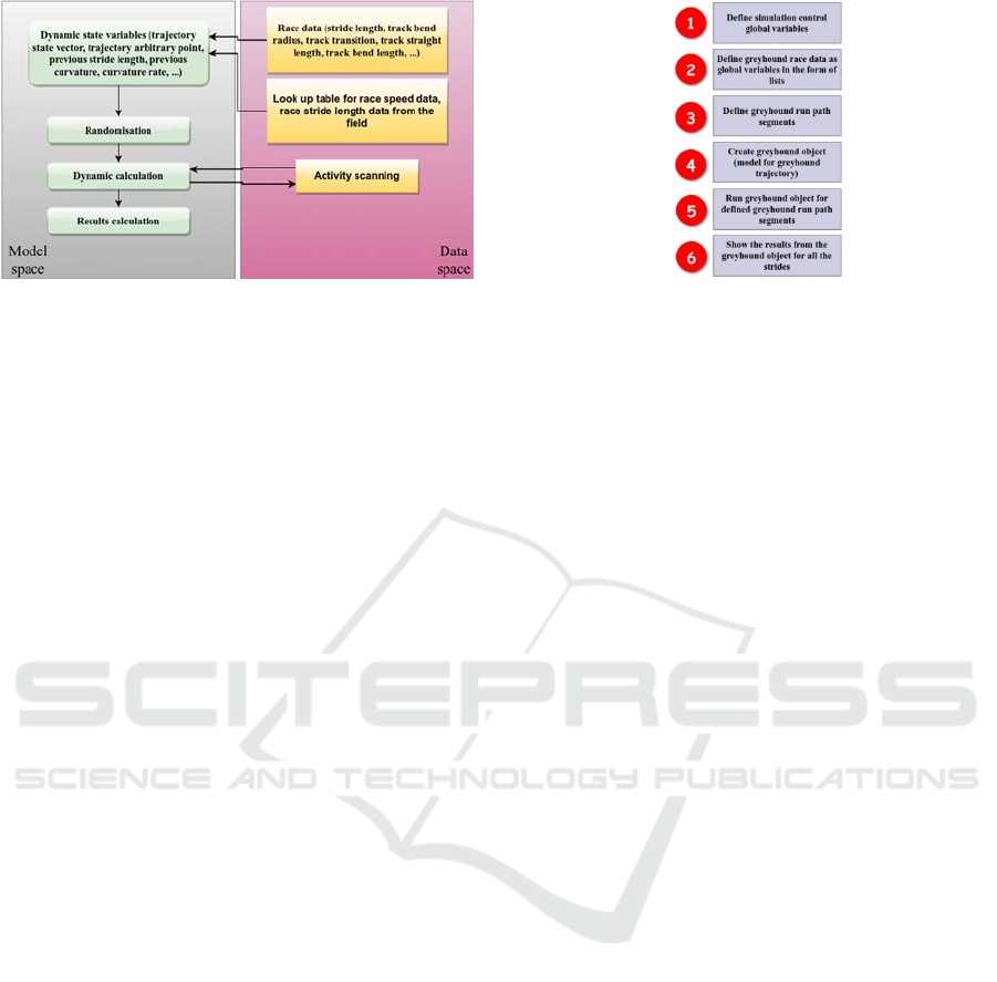
Figure 1: Primary components and their data sharing for
simulating greyhound dynamics at discrete stride points.
As this research is about greyhound trajectory
modelling using discrete strides as data and event
points, it only answers greyhound dynamic states
after each stride. Any intermediate conditions of
greyhound dynamics such as greyhound bumping
or crashing into an obstacle during a stride need
separate models which are not part of this research.
Thus, this research utilises greyhound dynamic
states such as curvature, and stride length from the
models to generate greyhound trajectory dynamics
such as jerk for different greyhound path following
conditions by applying the principle of discrete-
event simulation.
3 SIMULATION PLATFORM
Discrete-event simulators often time use their special
programming languages. Nowadays, general-purpose
programming languages are being utilized for
designing simulation programs (Liu et al., 2020). As
a general-purpose programming language Python is
known as versatile and has an error-free approach to
coding. The simulation for this research was carried
out in Python programming language. Python
variables and objects were used for storing different
simulation variables states and deriving results.
Python built-in and custom-built methods and
statements were used for randomising variables
assignments, creating simulation conditions, and
defining equations.
Figure 2 illustrates the main components in the
Python simulation module in order.
Figure 2: Steps followed for writing Python module for a
simulation.
4 GREYHOUND TRAJECTORY
FOR THE BEND
Greyhound location tracking data showed that
greyhounds follow a smooth continuous path
trajectory despite the track path being not optimised
for shape continuity. For instance, track bend and
straight sections meeting next to each other where
there is no proper smoothing curve applied would
result in a sudden change in centrifugal acceleration
requirement when moving from straight to the bend.
As data showed a continuous path of racing
greyhound it can be said that greyhound minimises
large variations of turn radius while navigating
around the track. Figure 2 illustrates the main
components in the Python simulation module in
order.
To validate greyhound run conditions in absence
of a proper track path transition curve between the
bend and straight three scenarios can be considered.
In all scenarios, greyhounds make a small transition
for entering the bend that would allow them to enter
the bend without hitting the track outside fence. It was
found in the data that greyhounds make a smaller turn
radius than the bend radius at different points on the
track. In the first scenario, the greyhound's transition
exit turn radius is smaller than the track bend radius
where the greyhound continues to follow a smaller
radius turn to align itself with the bend as shown in
Figure 3. In the second scenario, the greyhound
transition exit turn radius is the same as the track
bend, but the greyhound makes a smaller radius turn
after exiting the transition to align itself with the bend
as shown in Figure 4. In the third scenario, the
greyhound's transition exit turn radius is smaller than
the track bend radius where the greyhound continues
to follow the track bend radius after exiting the
transition to align itself with the bend as shown in
Simulating Theoretical Jerk by Numerical Modelling for Greyhound Racing
381

Figure 5. In Figures 3, 4 and 5 it can be seen that with
a 50% smaller turn radius than the bend radius
greyhound has a greater chance of aligning itself with
the bend in the lack of a track transition without
bumping into the track outside fence. With 65%
smaller turn radius than the bend only in the first and
second scenarios would allow the greyhound to align
with the bend as it gets very close to the track outside
Figure 3: Greyhound transitioning into the bend with no
track bend transition where the smallest radius turn is same
as the transition exit radius.
Figure 4: Greyhound transitioning into the bend with no
track bend transition where the smallest radius turn is not
same as the transition exit radius.
Figure 5: Greyhound transitioning into the bend with no
track bend transition where the smallest radius turn is the
transition exit radius.
fence. With a 75% smaller turn radius than the bend
only in the first scenario greyhound would be able to
continue to follow the track without bumping into the
track outside. Finally, all three scenarios would result
in different greyhound trajectory jerk outcomes based
on greyhound transition length, transition exit radius
and greyhound speed conditions.
4.1 Jerk Experienced by the
Greyhound for Entering the Bend
The following major greyhound kinematics variables
were analysed.
4.1.1 Influence of Speed
It is shown in the data that greyhound running speed
is decreased during entering the bend. As the
greyhound enters the bend it makes a transition from
the straight to the constant radius bend. During this
transition phase, the greyhound yaw rate changes
from a lower value to a higher value. From Eq. 2 of
yaw rate, we can see that if the yaw rate changes an
equivalent change in the greyhound speed is required
to balance the greyhound kinetic energy state. From
this equation, we can tell that a transition would force
the greyhound to slow down or decrease its speed for
entering the bend. Also, this implies that a non-
optimum transition would decrease greyhound speed
significantly where a high braking force is required
when entering the bend.
Speed =
y
aw rate * turnin
g
radius (2)
As centrifugal acceleration jerk is a function of
speed, a changing speed during entering the bend
would imply a changing jerk value. Also, greyhound
peak speed would vary based on the greyhound’s start
location distance from the bend which would also
affect the jerk outcome.
4.1.2 Influence of Stride Length
Greyhound stride length is responsible for increasing
its speed. Greyhound stride length can be described
by Eq. 3. With a variable stride length for entering the
bend, the requirements for turning radius and heading
yaw is different from a constant stride length during
bend transition. This also affects greyhound
centrifugal acceleration jerk as a result.
Speed = stride len
g
th * stride frequenc
y
(3)
SIMULTECH 2022 - 12th International Conference on Simulation and Modeling Methodologies, Technologies and Applications
382
4.1.3 Influence of Transition Length
For greyhound transition, we can assume an Euler
curve as it has a continuous linear centrifugal
acceleration profile where the centrifugal acceleration
is zero for the straight and peak at the transition exit
point. A longer Euler transition would decrease the
centrifugal acceleration jerk while a shorter one
would increase the jerk requirement.
4.1.4 Influence of Bend Radius
For oval shaped track, a constant radius bend is used
for creating the track loop along with straight sections
where track transition may or may not exist. A larger
bend radius would decrease jerk requirements in the
presence of a transition.
4.2 Jerk Outcome for Different
Greyhound Trajectories for the
Bend
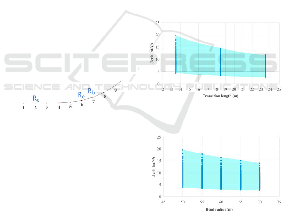
Numerical simulation was carried out by defining
major transition points for the greyhound trajectory
for entering the bend. The transition point between
straight and transition curve can be seen in Figure 6
as denoted by R
s
. The transition point between the
bend and transition curve is denoted by R
e
. Finally,
the bend radius point is denoted by R
b
.
Figure 6: Transition points on greyhound trajectory for
entering the bend where red dots are strides.
Now, for the scenarios explained in Section 4,
the relationship between transition exit radius
R
e
and bend radius R
b
are given below:
First scenario: R
e
= R
b
Second scenario: R
e >
R
b
Third scenario: R
e
< R
b
For generating the results three variables are
enumerated namely, start box distance from the bend,
track bend radius and transition length. Furthermore,
these variables are defined according to the existing
track designs. Finally, the limit for greyhound
transition length in the absence of track transition was
calculated by modelling existing smallest and largest
radius tracks by assuming no track transition is
applied. Thus, a minimum greyhound transition
length consisted of three strides. This is because a
minimum of three strides are required for heading
deflection angle change when it is assumed
greyhound changes its heading with every stride. The
maximum greyhound transition length for 70 m and
50 m radius bends are found to be 23.5 m and 20 m
respectively. This is because anything greater than
these values would make the greyhound bump into
the track outside fence for making the transition as
track transition is not present. The following sections
illustrate maximum jerk values for with and without
track transitions as produced from numerical
simulations.
4.2.1 Greyhound Make Own Transition
When there is no track transition path segment, the
greyhound still should be able to create its own
transition given that it does not bump into the track
outside fence. Figures 7 to 12 depict jerk outcome for
greyhound transition into the bend from the straight
Figure 7: Maximum jerk envelope for different greyhound
transition lengths from the first scenario simulations
depending on track bend radius and distance of the race start
from the bend.
Figure 8: Maximum jerk envelope for different bend radius
from the first scenario simulations depending on greyhound
transition length and distance of the race start from the
bend.
Simulating Theoretical Jerk by Numerical Modelling for Greyhound Racing
383

Figure 9: Maximum jerk envelope for different greyhound
transition lengths from the second scenario simulations
depending on track bend radius and distance of the race start
from the bend.
Figure 10: Maximum jerk envelope for different bend
radius from the second scenario simulations depending on
greyhound transition length and distance of the race start
from the bend.
Figure 11: Maximum jerk envelope for different greyhound
transition lengths from the third scenario simulations
depending on track bend radius and distance of the race start
from the bend.
for scenarios explained before. The figures show the
maximum jerk value envelope for greyhound's
different transition lengths and track bend radii. The
blue dots represent the simulation run results as
produced for different simulation scenarios.
Figure 12: Maximum jerk envelope for different bend
radius from third scenario simulations depending on
greyhound transition length and distance of the race start
from the bend.
4.2.2 Greyhound Follow Track Transition
When there is a track transition path segment it is
easier for the greyhound to hold its line and follow
approximately track transition. Figures 13 and 14
depict jerk outcomes for a greyhound following track
transition into the bend from the straight. The figures
show the maximum jerk value envelope for different
transition lengths and track bend radii. The blue dots
represent the simulation run results as produced for
different simulation scenarios.
Figure 13: Maximum jerk envelope from the simulations
for different Euler transition lengths path following
depending on track bend radius and distance of the race start
from the bend.
Figure 14: Maximum jerk envelope from the simulations
for different bend radius depending on Euler track transition
length and distance of the race start from the bend.
SIMULTECH 2022 - 12th International Conference on Simulation and Modeling Methodologies, Technologies and Applications
384

5 DISCUSSION
Numerical simulation of greyhound trajectory for the
bend predicted greyhound theoretical jerk outcome
by utilizing different parameters pertaining to
greyhound strides and track variables. As can be seen
from the maximum jerk value plots in the previous
section greyhound would experience different levels
of centrifugal acceleration jerk. For instance, jerk
levels are much higher when greyhounds followed
their own transitions despite the lack of track
transition as depicted in Figures 7 to 12. In the first
scenario, the jerk was lower than in the second and
the third scenarios. The second scenario resulted in
the highest jerk levels for all transitions and track
bend radii run conditions. In all three scenarios, the
highest jerk can go above 20 m/s3 for the lowest
transition length and turn radius while in the second
and third scenarios jerk remains greater than 20 m/s3
for all greyhound run conditions.
If greyhound followed a track transition with
continuous turn radius its jerk level is under 7 m/s
3
for
smallest transition and bend radius. Furthermore,
with optimal run conditions the 75 m transition peak
jerk remains between 1 and 2 m/s
3
as depicted in
Figure 13. However, when the run conditions are not
optimal a large radius bend will maintain the jerk
level between 1 and 5 m/s
3
as depicted in Figure 14.
6 CONCLUSIONS
This research showed greyhound racing centrifugal
acceleration theoretical jerk by modelling greyhound
stride dynamics based on data and numerical
simulation. By formulating various greyhound run
conditions for track bends and transitions this
research arrived at possible scenarios for greyhound
trajectories and corresponding significant jerk
outcomes. The results from the research showed the
theoretical jerk levels which greyhounds face during
various run conditions often time created by track
variables such as less than ideal track transition
design. Finally, this paper presents an idea about
analysing stride dynamics using numerical modelling
and simulation.
ACKNOWLEDGMENTS
This work is sponsored by the Faculty of Engineering
and Information Technology at the University of
Technology, Sydney, Australia. Special thanks to
Greyhound Racing Victoria, Australia for providing
real-time race data and track survey plans.
REFERENCES
Mahadavi F., Hossain I., Hayati H., Eager D., Kennedy P.,
Track shape, resulting dynamics and injury rates of
greyhounds, ASME-IEMCE 2018, Pittsburgh,
Pennsylvania, USA, 9-15 November 2018.
Hayati H., Eager D., Pendrill A-M., Alberg H. (2020). Jerk
within the context of science and engineering—A
Systematic Review. Vibration 2020, 3, 371-409.\\
doi:10.3390/vibration3040025
Pendrill, A-M., Eager D. (2020). Velocity, acceleration,
jerk, snap and vibration: forces in our bodies during a
roller coaster ride. Eur. J. Phy. 55(6) 065012.
doi:10.1088/1361-6552/aba732
Eager D., Pendrill, A-M., Reistad N. (2016) Beyond
velocity and acceleration: jerk, snap and higher
derivatives. Eur. J. Phy. 37(6) 065008.
\\doi:10.1088/0143-0807/37/6/065008
Hasti H., Eager D., Walker P. (2019). The effects of surface
compliance on greyhound galloping dynamics,
Proceedings of the Institution of Mechanical Engineers,
Part K: Journal of Multibody Dynamics, 233(4), 1033-
1043. doi:10.1177/1464419319858544
Hossain, M., Eager, D., Walker, P. D., et al. (2020).
Greyhound racing ideal trajectory path generation for
straight to bend based on jerk rate minimization.
Scientific Reports, 10(1):1–15.
Liu, J. (2020). Simulus: Easy breezy simulation in python.
In 2020 Winter Simulation Conference (WSC), pages
2329–2340. IEEE.
Simulating Theoretical Jerk by Numerical Modelling for Greyhound Racing
385
