Big Data Analysis of Ionosphere Disturbances using Deep Autoencoder

and Dense Network

Rayan Abri

1 a

, Harun Artuner

2 b

, Sara Abri

1 c

and Salih Cetin

1 d

Mavinci Informatics Inc., Ankara, Turkey

Department of Computer Engineering, Hacettepe University, Ankara, Turkey

Keywords:

Ionosphere, Total Electron Content, Deep Autoencoder, Deep Neural Networks, Linear Discriminant Analysis.

Abstract:

The ionosphere plays a critical role in the functioning of the atmosphere and the planet. Fluctuations and some

anomalies in the ionosphere occur as a result of solar ﬂares caused by coronal mass ejections, seismic motions,

and geomagnetic activity. The Total electron content (TEC) of the ionosphere is the most important metric

for studying its morphology. The purpose of this article is to examine the relationships that exist between

earthquakes and TEC data. In order to accomplish this, we present a classiﬁcation method for the ionosphere’s

TEC data that is based on earthquakes. Deep autoencoder techniques are used for the feature extraction from

TEC data. The features that were obtained were fed into dense neural networks, which are used to perform

classiﬁcation. In order to assess the suggested classiﬁcation model, the results of the classiﬁcation model are

compared to the results of the LDA (Linear Discriminant Analysis) classiﬁer model.The research results show

that the suggested model enhances the accuracy of differentiating earthquakes by around 0.94, making it a

useful tool for identifying ionospheric disturbances in terms of earthquakes.

1 INTRODUCTION

As it slowly rises above the ground, it encounters an

atmospheric taxonomy in terms of height, and some

of the atmospheric layers have several key properties.

The ionosphere layer is one of the most signiﬁcant

layers in the atmosphere, with numerous unique prop-

erties. These characteristics help to identify a wide

range of events, such as solar ﬂares and earthquakes.

The ionosphere layer, which extends from 48 km to

960 km and is ionized into a plasma phase.

Total Electron Content is a primary quantiﬁable

statistic that identiﬁes an ionosphere property (TEC).

TEC is a powerful tool for studying the ionosphere’s

morphology. TEC is described as the line integral of

electron density along a ray path or a metric of to-

tal electrons across a ray path in the literature. TEC

is measured in TECUs (TEC Units), with 1 TECU

equaling 1016 electron/m2 as described by (Arikan

et al., 2003)(Nayir et al., 2007). Measuring and moni-

toring TEC Values can describe the ionosphere layer’s

https://orcid.org/0000-0002-2787-2832

https://orcid.org/0000-0002-6044-379X

https://orcid.org/0000-0001-6637-9787

https://orcid.org/0000-0002-9501-7192

variations and turbulences effectively and efﬁciently.

According to (Nayir et al., 2007), the Global Po-

sitioning System (GPS) has provided a cost-effective

approach in estimating and analyzing TEC and mon-

itoring the ionospheric layer disruptions across a sig-

niﬁcant fraction of the global continent during the last

several decades. The temporal and geographical vari-

ability of the ionosphere layer is closely related to

the earth’s daily (every day) and yearly rotation, as

well as the pattern of magnetic ﬁeld lines of the ge-

omagnetic dipole. Even when there are no geomag-

netic events, the earth’s magnetic ﬁeld is not silent, as

(Rishbeth and Garriott, 1969) describes. Fluctuations

in geomagnetic and solar activity, as well as seismic-

ity, affect the ionosphere’s quiet circumstances. As

a result, these repercussions may produce changes in

parameters such as earthquakes.

In summation, this paper offers a model based on

deep learning approaches for interpreting the link be-

tween earthquakes and ionosphere perturbations, with

two sub-tasks of feature extraction and classiﬁcation.

The model’s initial phase focuses on using Deep Au-

toencoders and unsupervised learning approaches to

extract features from TEC data. The suggested clas-

siﬁcation using deep dense neural networks based on

the supervised learning approach is the second step.

158

Abri, R., Artuner, H., Abri, S. and Cetin, S.

Big Data Analysis of Ionosphere Disturbances using Deep Autoencoder and Dense Network.

DOI: 10.5220/0011332900003269

In Proceedings of the 11th International Conference on Data Science, Technology and Applications (DATA 2022), pages 158-167

ISBN: 978-989-758-583-8; ISSN: 2184-285X

The following is the rest of the story. The related

works on Total Electron Content variation produced

by magnetic and earthquake disruptions in the iono-

sphere layer are discussed in Section 2. The iono-

spheric dataset and prepossessing stages for the pro-

posed models are presented in section 3. In Section

4, we show our classiﬁcation model for ionospheric

data. Sections 5 and 6, respectively, cover the eval-

uation technique and outcomes. The ﬁnal comments

and future studies are found in section 7.

2 RELATED WORK

The relevant studies for observing ionospheric pertur-

bations are presented in this section. Geomagnetic

events such as storms and earthquakes may cause se-

vere disruptions in the electron density distribution.

The seismo-ionospheric anomalies as stated by (Pu-

linets et al., 2018; Tao et al., 2017) have been inves-

tigated using satellite-based observations from GPS

stations.

The ionospheric disruption and storms may cause

severe turbulence in the ionosphere’s TEC values was

explored by (Biqiang et al., 2007; Trigunait et al.,

2004). Furthermore, earthquakes and seismic activ-

ity, according to (Pulinets et al., 2003), might produce

changes in electromagnetic signals and the chemical

properties of the atmosphere in the troposphere, and

ionosphere.

Many studies, such as those cited in (Liu et al.,

2004; Le et al., 2011; Liu et al., 2006; Liu et al.,

2010), concentrate on statistical evaluations of the

empirical association between ionospheric based ab-

normalities and earthquakes. For example, in (Liu

et al., 2004), the authors looked at the TEC associ-

ated with 20 strong (Magnitude ≥ 6.0) earthquakes

in Taiwan over the course of four years (1999–2002).

During the other quiet days, they discover irregulari-

ties that show the TEC value is decreasing ﬁve days

before the earthquakes. Furthermore, (Le et al., 2011)

shows the relationship among TEC-based ionospheric

abnormalities and severe earthquakes (Magnitude

≥ 6.0) throughout a nine-year period (2002–2010).

They also veriﬁed that earthquakes with a strength of

≥ 7.0 and a depth of ≤ 20 km cause a high percentage

of anomalies in the ionosphere.

(Ulukavak and Yalcinkaya, 2017; Pundhir et al.,

2017; Oikonomou et al., 2016) have recently ob-

served aberrant ionospheric layer changes based on

TEC values measured days and hours before severe or

large earthquakes. The data for the TEC was collected

from a GPS station in the earthquake zone. There

are some questions concerning how to create such

anomalies near the epicenter of powerful earthquakes.

According to (Tariq et al., 2019), and (Shah and Jin,

2015), there are direct links between ionosphere va-

riety and earthquakes. TEC values acquired from

the GPS receiver varied and rose before Magnitude

≥ 6.0 earthquakes occurred throughout the period

1998–2014. According to the authors of (Le et al.,

2011), ionospheric TEC abnormalities were used to

categorize severe and strong earthquakes based on

their magnitudes.

We plan to extract signiﬁcant aspects of earth-

quakes using TEC values in the ionosphere layer,

and then identify earthquake days in the target sta-

tion zone, based on previous research in this area.

Our main emphasis is on extracting characteristics

from earthquakes and classifying them using TEC

data from the ionospheric. We are not focusing on

forecasting earthquakes in previous days at this time,

and our study is focused on TEC changes during mod-

erate and severe earthquakes.

3 DATASET AND DATA

PREPRATION

The dataset relating to earthquakes and GPS station

TEC values was introduced in this part. The proce-

dures for preparing the dataset are also described.

3.1 Dataset

TEC values derived from GPS stations, as described

in Section 2, are a valuable approach to assessing the

ionospheric reaction to earthquakes and solar storms.

The ionospheric variability is investigated using TEC

data collected from GPS stations (Dual-Frequency

GPS receiver). TEC data was acquired from two

GPS sites for this study. This information was gath-

ered from the IONOLAB group (Hacettepe Univer-

sity of IONOLAB is an organization of electrical

engineers to investigate hurdles of the ionosphere.)

. The ﬁrst station is placed at coordinates (Lat :

−20.15,Lon : −70.13) Figure 1 shows the city of

Iquique in Chile. The second station is located at co-

ordinates (Lat : −20.85, Lon : 117.1) Figure 1 depicts

Karratha, a town in Western Australia’s Pilbara area.

The earthquake data is gathered by the (United States

Geological Survey of Earthquakes)

This research examines ionospheric ﬂuctuation

across moderate and severe earthquake occurrences

of varied magnitudes from 2012 to 2019. The data

Available at http://ionolab.org/

Available at https://earthquake.usgs.gov/

Big Data Analysis of Ionosphere Disturbances using Deep Autoencoder and Dense Network

159

Figure 1: The Iquique (Chile) and station and the Karratha

(Western Australia) station.

Figure 2: The Iquique and Karratha stations located in the

same latitude from the two hemispheres of the east and west

of the earth.

for each station was gathered between 2012 and 2019.

The data was divided day by day with 2880 TEC sam-

ples in a day. The stations are positioned in the same

latitude from the east and west hemispheres of the

earth, as shown in Figure 2. The Chile area is known

to powerful and severe earthquakes, however the Kar-

ratha region is rather earthquake-free.

3.2 Data Preparation

The reliability of the input dataset is crucial in deep

learning ideas because there is a direct link between

the reliability of the input data and the effectiveness of

the trained model. Data preprocessing includes data

tuning procedures that transform raw input data into

a usable format. Ionospheric TEC data is often inad-

equate, inconsistent, and prone to many inaccuracies.

In this study data preprocessing is divided into three

stages: cleaning, transformation, and reduction.

The cleaning stage aims to delete missing values

and perform regressions using previous and later ob-

servations samples to smooth noisy values since raw

TEC data on certain days has missing and noisy val-

ues. Furthermore, the gathered data is transformed

into suitable mining formats. TEC data are scaled to

a speciﬁc deﬁned range to accomplish the normaliza-

tion (0,1.0). A day’s value of TEC data contains of

2800 samples. Learning enormous volumes of input

data with various characteristics in data mining makes

analysis problematic or impossible, and the training

process might take a long period of time. Data Re-

duction is a collection of approaches for reducing the

number of input samples in a dataset without harm-

ing the integrity of the original data. A single day’s

data is reduced from 2800 to 95 by sampling TEC

values every ﬁfteen minutes. The ionospheric and

EQs(earthquakes) datasets are detailedly described in

Table 1. All of the earthquakes were recorded at sta-

tions within a 250-kilometer radius.

The gathered data is shown in the table as well as

information such as the ratio of the train and test sets.

Table 1: Detailed information of the dataset.

Dataset Characteristics Value

Day count in uncleaned Dataset 2922

Day count in cleaned Dataset 2571

Train-Test Ratio 80%-20%

Total EQs≥4.5 141

Total EQs≥5.0 91

Day count in Trainset 2057

Day count in Testset 514

EQs ≥4.5 in Trainset 113

EQs ≥5.0 in Trainset 73

EQs ≥4.5 in Testset 28

EQs ≥5.0 in Testset 18

Solar ﬂares and other cosmological event compo-

nents have been shown to inﬂuence the ionosphere in

early research. Xray ﬂuxes are increased during solar

ﬂares, and this has been recognized as the source of

increased ionization in the ionosphere. Although, this

research focuses on ionospheric changes and TEC

ﬂuctuations during various earthquakes, it is neces-

sary to diminish the impact of solar ﬂares and other

cosmological events in order to identify earthquakes

and geomagnetic activity more accurately.

As previously stated, the stations are placed at

the same latitude as the earth’s east and west hemi-

spheres. Because solar ﬂares and other comparable

cosmic occurrences inﬂuence both the east and west

hemispheres of the planet, the similarity between two

places may be estimated. Solar ﬂares and other such

cosmic occurrences are shown by anomalies on the

same day in both the stations. It is possible that the

related stations contain the same irregularities as a re-

sult of solar ﬂares and other cosmic phenomena. To

reduce the impact of these abnormalities, it is neces-

sary to compute the similarity between the stations.

The similarity among coincident days at each re-

gion in the dataset is calculated for this objective. Be-

cause of the structure of the dataset, the similarity be-

tween coinciding days at each station is estimated us-

ing cosine similarity. Cosine similarity is a measure

that compares two non-zero vectors and is deﬁned by

the cosine of their angles. Equation 1 is used to com-

pute the cosine similarity.

cos(x,y) =

x.y

∑

i=1

∑

i=1

∑

i=1

(1)

DATA 2022 - 11th International Conference on Data Science, Technology and Applications

160

Where x and y are the TEC data vectors for each

day in the stations.

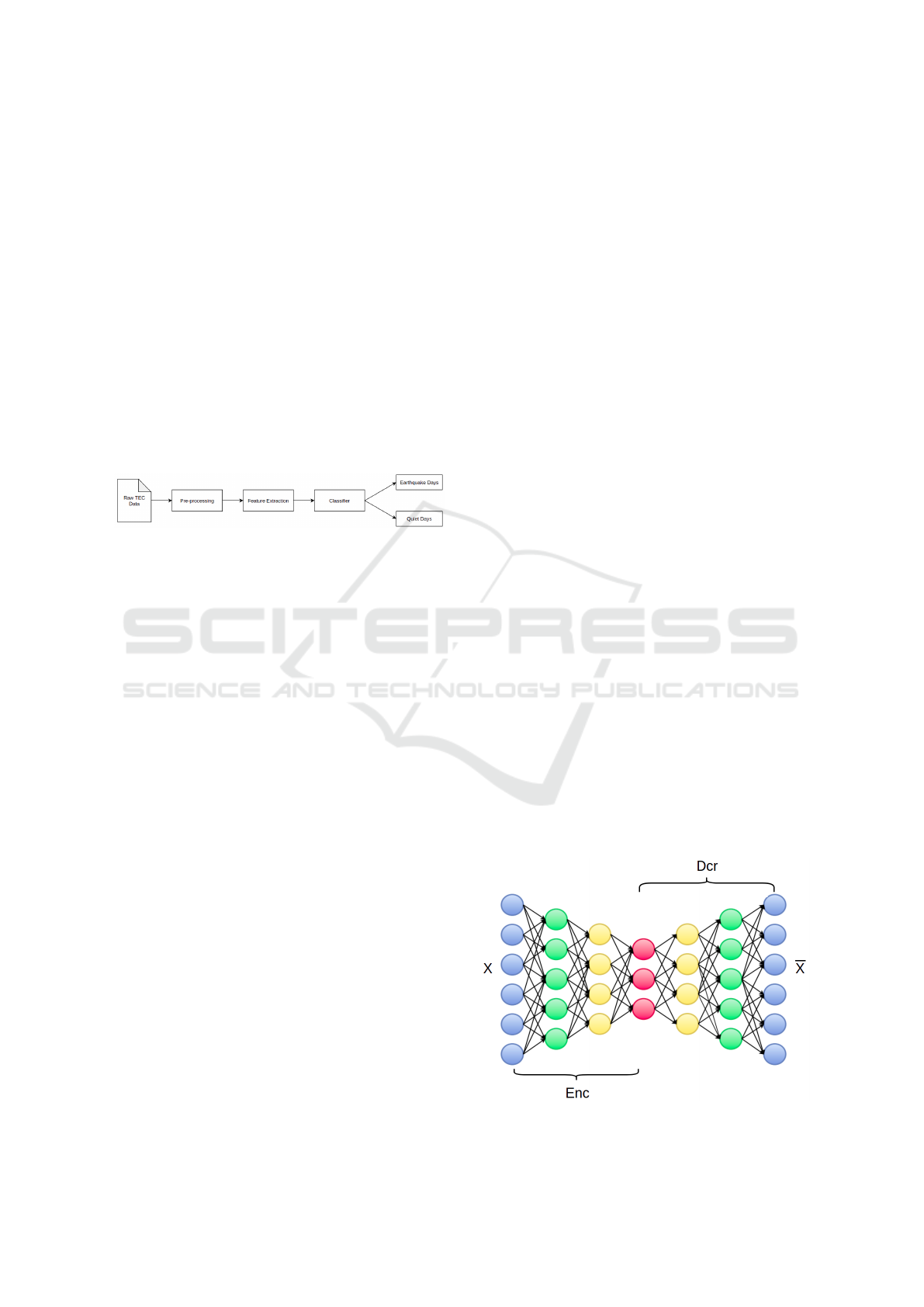
4 METHOD

The framework of the suggested model is given in this

section. A broad overview of the suggested model is

shown in Figure refﬁg:model. Deep neural networks

are utilized because of the vast quantity of TEC data

associated with each station. Because Deep Learn-

ing’s core beneﬁt is the study and learning of huge

volumes of supervised and unsupervised data, it’s par-

ticularly useful for Big Data Analytics, where data

is mostly unlabeled. Unsupervised learning methods

such as Deep Autoencoders and deep dense networks

are employed in the proposed model.

Figure 3: Overview of the proposed model.

4.1 Feature Extraction

The main feature extraction techniques presented by

(Khalid et al., 2014) are based on projection and data

mapping from a complicated input space with many

dimensions to a new output space with fewer dimen-

sions while minimizing data loss. (Dem

sara et al.,

2013; Sharma and Paliwal, 2015) discuss two promi-

nent projection methods: Principal Component Anal-

ysis (PCA) and Linear Discriminant Analysis (LDA).

The PCA technique projects the input data into its pri-

mary directions by maximizing variance. This tech-

nique is classiﬁed as an unsupervised technique. The

LDA, on the other hand, optimizes discriminating

data from input classes in order to produce a linear

output space. The LDA technique is characterized

as a supervised learning technique. The fundamental

difﬁculty with the techniques outlined is linear pro-

jection. (Lopez-Paz et al., 2014) propose non-linear

kernel functions as a solution to this problem.

Due to the large dimensionality of ionospheric

TEC data, lowering dimensionality to create a com-

pressed feature set is considered an important step in

the feature extraction process. Traditional machine

learning algorithms should theoretically be capable

of operating on any number of characteristics. These

models with large-dimensional datasets are exposed

to issues like as over-ﬁtting of the training set, exces-

sive computational cost, and the dimensionality curse.

Autoencoders use neural networks to reduce the input

dimensions, with the goal of minimizing reconstruc-

tion loss. As a result, adding hidden layers to the au-

toencoders causes the dimension reduction process to

work properly. Deep Autoencoders have been shown

to be successful in detecting non-linear features in a

variety of scenarios.

Deep Autoencoders are multi-layer neural net-

works that produce the desired output from the input.

Within a pair of encoding and decoding steps, an au-

toencoder learns a map from the input to itself. For

feature learning, autoencoders have recently directed

to unsupervised approaches. It attempts to learn a

condensed description of the input while maintaining

the most critical data.

X = Dcr(Enc(X)) (2)

Where X represents the input TEC data, Enc rep-

resents an encoding map from the TEC data to the

hidden layer, Dcr represents a decoding map func-

tion from the code layer to the output layer, and barX

represents the recovered a similar version of the TEC

data in Equation 2. The goal is to teach Enc and

Dcr to reduce the difference between X and barX as

much as possible. To reduce the error of reconstruc-

tion of input from hidden code nodes, the encoder and

decoder functions (Enc and Dcr) are trained concur-

rently. An autoencoder might be seen as a possible

reason for the optimization issues.

min

Dcr,Enc

k X −Dcr(Enc(X )) k (3)

In Equation 3, k . k is commonly considered to be the

− norm.

The input, encoder, decoder, and output layers are

shown in Figure 4. The autoencoder may output a

more compact vector as input vector if the reconstruc-

tion error is reduced. Sigmoid and ReLU, as deﬁned

in Equations 4 and 5, are employed in this study.

Figure 4: A Deep Autoencoder with ﬁve layers.

Big Data Analysis of Ionosphere Disturbances using Deep Autoencoder and Dense Network

161

ϕ(z) =

1 + e

−z

(4)

R(z) = max(0,z) (5)

The output of the x

node in the i

layer is obtained

sequentially from the output of the prior nodes in the

previous layer as Equation 6 where bias

is bias scalar

and N

represents the number of nodes in the i

layer,

x,n

is the weights which connect the x

node in the

layer to the n

node in previous layer.

= ϕ(net

) = ϕ(

i−1

∑

n=1

x,n

(i−1)

+ bias

) (6)

Increasing the number of layers improves the ca-

pacity to learn more complex patterns. The matrix of

all weights W is changed to minimize the mean square

error over the training set, as shown in Equation.

ε =

∑

i=1

k X −Dcr(Enc(X )) k

(7)

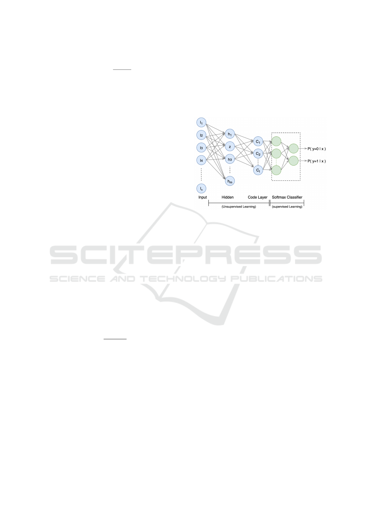
4.2 Classiﬁcation Method

After the feature extraction, these features must be

classiﬁed. Several different classiﬁcation methods

have been used in the literature. Deep neural networks

are often used in combination with softmax regres-

sion. It is possible to combine the classiﬁer and en-

coder functions for this purpose. Logistic regression

is induced by softmax (multinomial logistic) regres-

sion. It uses Equation 8 to calculate the probability of

the i

class.

Prob

= Prob(i|I) =

∑

n=1

i = 1,...,N (8)

Where w

are the training weights for the i

class and

I is the classiﬁer’s input. The classiﬁcation is carried

out by comparing Prob

’s. The softmax may simply

be used with the encoder function to form the net-

work’s deep structure.

Figure 5 shows a block diagram of the suggested

autoencoders. It’s a combined model that includes

both unsupervised and supervised learning. The en-

coder that was learned in the feature extraction step is

used for unsupervised learning, while the supervised

model is a dense softmax classiﬁer.

By decreasing the error rate and employing Equa-

tion 7, features at hidden layer two are reduced and

compressed. These characteristics are then supplied

to the next autoencoder layer, and the features from

layer three (code layer) are fed to the softmax classi-

ﬁer, which uses labeled data to do classiﬁcation. Dur-

ing the feature extraction step, the layers of the Deep

Autoencoder are trained individually. As a result, the

features are learnt unsupervised, whereas classiﬁca-

tion is done supervised.

Figure 5: The structure of the proposed model.

5 EVALUATION

METHODOLOGY

By using learning parameters and evaluation metrics

discussed in this section, you will be able to better

grasp the metrics necessary to conduct a quality as-

sessment.

As previously noted in Section 4; the TEC val-

ues are split by days and classiﬁed using the sug-

gested model in the technique section, as previously

described. The suggested model is broken into two

sub-models, which are described below. The Deep

Autoencoder is used to extract the features from TEC

values in terms of days in the ﬁrst sub-model. When

the feature extraction phase is trained, it provides

a low-dimensional form that encodes a meaningful

topological structure of TEC characteristics in order

to reconstruct the high-dimensional input. The sec-

ond kind of dense network is a softmax dense net-

work, which is pinned to the encoder and is used to

do classiﬁcation jobs. The hidden layers of the clas-

siﬁer are bound by the earthquake labels in the data.

By combining the autoencoder with the classiﬁer, the

networks are trained.

When evaluating the performance of a model,

it is necessary to use model assessment measures.

The model determines which evaluation measures are

used and which ones are not. As a result of the nature

of the data and the suggested model, we employ the

accuracy, precision, and recall of the model as perfor-

DATA 2022 - 11th International Conference on Data Science, Technology and Applications

162

mance indicators. The accuracy of classiﬁcation mod-

els is a frequent assessment parameter in this context.

It is deﬁned as the ratio of the number of correctly

identiﬁed earthquakes to the total number of correctly

classiﬁed days. Precision deﬁned as the ratio of accu-

rately identiﬁed earthquake days to the total number

of days labeled as earthquake days in a year. The re-

call is a measure of how well our model performs in

properly detecting earthquake days when compared to

the total number of earthquake days. Depending on

the data and requirements of the classiﬁcation model,

it may be necessary to prioritize precision and recall

over the other. The nature of this study is the cate-

gorization of ionosphere disturbances based on earth-

quakes. In addition to earthquakes, ionospheric dis-

turbances may inﬂuence other types of phenomena.

Therefore, the number of false positives may be ac-

ceptable in the classiﬁcation model.

A relationship or trade-off exists between preci-

sion and recall values in conventional classiﬁcation

models. The term ”F1-score” refers to a measure of

test set efﬁciency that takes into account both preci-

sion and recall while calculating the score. The F1-

score is the harmonic average of precision and recall

in Equation 9.

–score = 2 ∗

precision ∗ recall

precision + recall

(9)

It is possible to forecast the performance of ma-

chine learning algorithms by dividing a dataset into

two parts: the train set and the test set. As shown in

Table 1, the dataset has been divided into two groups:

train sets and test sets, with an 80-20 split ratio be-

tween the two groups. It seems that there is no appro-

priate ratio between the number of quiet days and the

number of earthquake days in the dataset.

As a consequence, there are only 141 earthquakes

with magnitudes greater than or equal to 4.5 between

2012 and 2019. A limited number of earthquake

classes are provided in the classiﬁcation model. With

just a limited number of earthquake classes included

in the classiﬁcation model, this results in an issue

known as imbalanced classiﬁcation, which is a dif-

ﬁculty in the model. When a class is relatively rare in

comparison to other classes, the class imbalance issue

emerges. There have been several approaches devel-

oped for unbalanced classiﬁcation by (Makki et al.,

2019; Lin et al., 2020), and some beneﬁcial ﬁndings

have been published in the literature.

In order to deal with the issue of unbalanced

classes, K-fold cross-validation has been used. In the

k-fold cross-validation approach, model performance

is evaluated by splitting the data into n equal folds and

then measuring the performance of the model on each

fold. This technique is similar to that of the repeated

random sampling technique. In an unbalanced class

distribution situation, the proper use of k-fold cross-

validation needs the usage of stratiﬁed k-fold cross-

validation, which is described below. In particular, it

has the ability to divide arbitrarily in such a manner

that the same class distribution is maintained in each

subset. Testing is carried out using a ten-fold cross-

validation strategy for the purpose of analyzing the

days. In order to make each fold a suitable sample of

the original dataset, 10 equal folds are randomly split

into the original dataset.

To determine the signiﬁcance of the suggested

combination model, we employed an LDA (Linear

Discriminant Analysis) classiﬁer based on the com-

pression of the features, similar to the work done by

the authors (Kim et al., 2011; Tharwat et al., 2017).

Linear discriminant analysis is implemented with the

aid of a max function M, which serves as a classiﬁca-

tion rule.

(X) =

(2p)

∑

exp

−

(X −µ

)

−1

∑

(X −µ

)

(10)

M(X) = X

−1

∑

−

−1

∑

+ log(p

) (11)

(X) represents the conditional density of X in

class i, where p

is the probability of class i. If the

vector of features X is variable and distributed with

a mean vector µ

and a shared covariance matrix

∑

then the solution is as follows: Once f

(X) has been

determined, as indicated in Equation 10, f

(X) may be

calculated. Calculation of the discriminant function

M(X) is done using the Bayes rule, which results in

Equation 11.

6 EVALUATION RESULTS

The performance of our suggested model, DAEclass

(Deep Autoencoder Classiﬁer), as well as the LDA

classiﬁer model, is assessed using the evaluation ap-

proach stated in Section 5. Speciﬁcally, the purpose

of this section is to evaluate and analyze the perfor-

mance metrics of both the suggested classiﬁcation

model and the LDA classiﬁer.

Table 2 gives the percentage of performance mea-

sures such as accuracy, recall, precision, and F1-score

for the proposed DAEclass model and LDA classi-

ﬁer based on two datasets. On the ﬁrst and second

Big Data Analysis of Ionosphere Disturbances using Deep Autoencoder and Dense Network

163

Table 2: Comparison of DAEclass and LDA classiﬁcation models using performance metrics.

Model Accuracy Precision Recall F1-Score

DAEclass-EQs≥4.5 0.93 0.56 0.75 0.64

LDA-EQs≥4.5 0.89 0.30 0.63 0.40

DAEclass-EQs≥5.0 0.96 0.61 0.83 0.70

LDA-EQs≥5.0 0.94 0.35 0.71 0.47

rows, you can see a comparison between the pro-

posed model and the LDA classiﬁer model, which

is based on all earthquakes with a magnetite ≥ 4.5

value in their dataset. It is undeniable that the sug-

gested model outperforms the LDA classiﬁer across

the board in all criteria. The suggested model im-

proved its precision and recall over the LDA classi-

ﬁer. The ﬂuctuations in the ionosphere layer are a re-

ﬂection of all cosmic and seismic activity. Precision

is lower than recall and accuracy because the false

positive count is high high owing to the unbalanced

classes in the dataset. The ﬁnal two rows compare the

proposed model to the LDA model, which is based

on more powerful earthquakes (magnetite-EQs ≥ 5.0)

than those in the ﬁrst two rows. Because severe earth-

quakes have a greater impact on the ionosphere than

mild earthquakes, they are more clearly characterized.

The performance difference between the two models

is lower than the performance gap between the two

models on the EQs≥ 4.5 dataset.

EQs≥4.5 and EQs≥5.0 datasets are represented

by the bar chart in Figure 6, which shows the com-

parison of performance measures between two mod-

els. It can be observed in Figure 6 (A) that the accu-

racy of the DAEclass increases marginally in the two

datasets that have been described. Precision and recall

measures are helpful indicators of classiﬁcation per-

formance when the classes are unequally distributed

over the dataset. As a consequence of earthquakes

and false alarms, precision is a measure of classiﬁ-

cation result relevance, while recall is the classiﬁer’s

capacity to locate all of the earthquake days. The

performance of the DAEclass classiﬁer is more sta-

ble when compared to the LDA classiﬁer, as shown

by the comparison of the two databases. Overall, the

DAEclass technique signiﬁcantly improves precision,

recall, and F1-score, as shown in Figure 6 (B)(C)(D).

This results in a greater extent of better performance

in the dataset EQs≥4.5 than the dataset EQs≥5.0, and

the DAEclass is more trustworthy in all earthquakes

as a result of this.

For the purpose of comparing multiple classiﬁers,

it might be advantageous to summarize the perfor-

mance of each classiﬁer into a single metric. The

Receiver Operating Characteristic (ROC) curve is a

commonly used and standard metric for comparing

various classiﬁcation models. It is calculated by com-

puting the area under the curve. The relationship be-

tween the true-positive rate and the false-positive rate

was shown by the receiver operating characteristic

curve (ROC curve).

Classiﬁers that produce curves that are closer to

the top-left corner of the screen demonstrate more de-

pendable performance. The ROC curves for the DAE-

class and LDA classiﬁer models, which were con-

structed using two datasets, are shown in Figure 7.

Because the ROC curves associated with the DAE-

class are positioned increasingly closer to the upper

left angle in ROC space, the DAEclass has a grad-

ually more signiﬁcant discriminant ability for earth-

quake classiﬁcation as time goes on. As shown in the

image, the DAEclass and the LDA classiﬁer may be

visually compared at the same time, with the results

indicating that the DAEclass is more efﬁcient than the

LDA classiﬁer in this case.

In order to evaluate the intrinsic performance of

classiﬁcation models, the AUC (area under the curve)

is an effective and integrated measure of the true-

positive and false-positive rates. In other words, the

bigger AUC indicates that the diagnostic test is ideal

for distinguishing between earthquake and quiet days.

The outputs are shown in Table 3, which shows the

AUC values of the model for each of the datasets.

The AUC in the DAEclass-EQs≥4.5 classiﬁer is 0.89,

while the AUC in the LDA-EQs≥4.5 classiﬁer is 0.79,

indicating a signiﬁcant increase in the ROC metric

in both classiﬁers. On the dataset EQs≥5.0, the

AUC values for the DAEclass technique are some-

what higher than those for the LDA classiﬁer, ranging

from 0.85 to 0.91.

Table 3: AUC values for the DAEclass and the LDA classi-

ﬁer.

Model ROC AUC

DAEclass-EQs≥4.5 0.892

LDA-EQs≥4.5 0.794

DAEclass-EQs≥5.0 0.914

LDA-EQs≥5.0 0.856

A statistical test is used to examine the suggested

model in further detail, in order to determine its de-

gree of signiﬁcance and potential for improvement. In

the test, the null hypothesis assumes that there is no

difference between the categorized earthquake days

DATA 2022 - 11th International Conference on Data Science, Technology and Applications

164

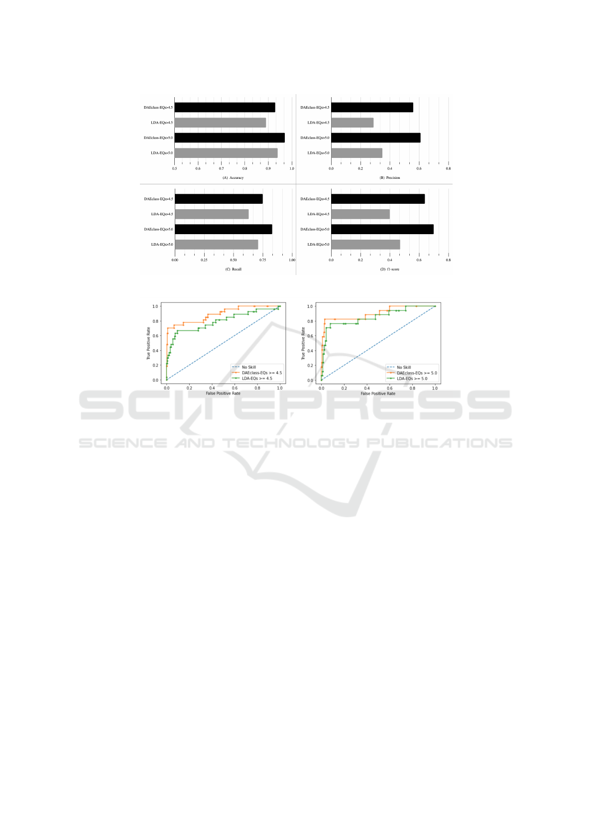
Figure 6: Performance metrics of the DAEclass and the LDA models based on two datasets (EQs≥ 4.5 and EQs≥ 5.0).

Figure 7: ROC curve of the DAEclass and the LDA classiﬁer models based on two datasets (EQs≥4.5 and EQs≥5.0).

and the quiet days. In order to determine whether or

not the null hypothesis under consideration can be re-

jected, the p-value test is done. The probability of de-

tecting the effect(E) when the null hypothesis is true is

represented by the P-Value. As shown by the test re-

sults of the DAEclass model, the difference in perfor-

mance across all measures is statistically signiﬁcant

(p − value  0.01).

7 CONCLUSION

This study presents a method for interpreting earth-

quakes based on TEC values in the ionospheric layer.

Data on ionospheric TEC was gathered from two

GPS sites. The Chilean area is prone to powerful

and severe earthquakes, however the Karratha region

is rather earthquake-free. The primary goal of this

study is to establish a link between earthquakes and

ionosphere disturbances using deep learning methods

to accomplish two sub-tasks: feature extraction and

classiﬁcation. Deep learning techniques are used to

accomplish this goal. In the ﬁrst stage, we concen-

trate on feature extraction from the TEC data, which

is accomplished via the use of an unsupervised learn-

ing algorithm. To extract relevant information about

the earthquake and quiet days, we create a Deep Au-

toencoder. Then, in the following stage, we use a su-

pervised learning approach to do classiﬁcation using

a dense neural network, which is followed by a ﬁ-

nal step. The LDA classiﬁer was used to examine

the contribution of the proposed combination model

to the overall contribution. Our ﬁndings show that

the two test sets of earthquakes, which included mild

and severe earthquakes, performed roughly 90-94 per-

cent accurately based on the correctness of the data.

In terms of accuracy, recall, precision, F1-score, and

ROC curve metrics, the proposed DAEclass outper-

forms the LDA in a more trustworthy and dependable

manner.

Because the primary purpose of this study is to ex-

tract important aspects of earthquakes from the iono-

sphere layer using TEC values and to identify earth-

quake days in the target station zone, earthquake pre-

diction is not within the scope and priority of this re-

search. In our other work (Abri and Artuner, 2022),

we planed to work on a predictive system to predict

earthquake using TEC data related to the earlier days

of earthquakes by LSTM based deep learning models.

Big Data Analysis of Ionosphere Disturbances using Deep Autoencoder and Dense Network

165

ACKNOWLEDGMENT

This research is supported by Mavinci Informatics

Inc. in Turkey, an R&D company in information and

communication technologies, security and defense ar-

eas with the capability of software development, arti-

ﬁcial intelligence, and machine learning. This article

is a thesis article and produced from the Ph.D. thesis

(Abri, 2021).

REFERENCES

Abri, R. (2021). Modeling of the ionosphere’s disturbance

using deep learning techniques. Hacettepe University,

Graduate School of Science and Engineering.

Abri, R. and Artuner, H. (2022). Lstm-based deep learn-

ing methods for prediction of earthquakes using iono-

spheric data. Gazi University Journal of Science.

Arikan, F., Erol, C. B., and Arikan, O. (2003). Regular-

ized estimation of vertical total electron content from

global positioning system data. In Proceedings of

American Federation of Information Processing So-

cieties: 1977 National Computer Conference, number

108.

Biqiang, Z., Weixing, W., Libo, L., and Tian, M. (2007).

Morphology in the total electron content under ge-

omagnetic disturbed conditions: results from global

ionosphere maps. Annales Geophysicae. Copernicus

GmbH, 25(7):1555–1568.

Dem

sara, U., Harris, P., Brunsdon, C., Fotheringham, A. S.,

and McLoone, S. (2013). Principal component analy-

sis on spatial data: an overview. Annals of the Associ-

ation of American Geographers, 103(1):106–128.

Khalid, S., Khalil, T., and Nasreen, S. (2014). In A survey of

feature selection and feature extraction techniques in

machine learning, 2014 science and information con-

ference, pages 372–378, London, UK. IEEE.

Kim, K. S., Choi, H. H., Moon, C. S., and Mun, C. W.

(2011). Comparison of k-nearest neighbor, quadratic

discriminant and linear discriminant analysis in clas-

siﬁcation of electromyogram signals based on the

wrist-motion directions. Current applied physics,

11(3):740–745.

Le, H., Liu, J.-Y., and Liu, L. (2011). A statistical analy-

sis of ionospheric anomalies before 736 m6. 0+ earth-

quakes during 2002–2010. Journal of Geophysical

Research: Space Physics, 116(A2).

Lin, E., Chen, Q., and Qi, X. (2020). Deep reinforcement

learning for imbalanced classiﬁcation. Applied Intel-

ligence, 50(8):2488–2502.

Liu, J. Y., Chen, C. H., Chen, Y. I., Yang, W. H., Oyama,

K. I., and Kuo, K. W. (2010). A statistical study of

ionospheric earthquake precursors monitored by us-

ing equatorial ionization anomaly of gps tec in taiwan

during 2001–2007. Journal of Asian Earth Sciences,

39(1-2):76–80.

Liu, J.-Y., Chen, Y. I., Chuo, Y. J., and Chen, C.-S.

(2006). A statistical investigation of preearthquake

ionospheric anomaly. Journal of Geophysical Re-

search: Space Physics, 111(A5).

Liu, J. Y., Chuo, Y. J., Shan, S. J., Tsai, Y. B., Chen,

Y. I., Pulinets, S. A., and Yu, S. B. (2004). Pre-

earthquake ionospheric anomalies registered by con-

tinuous gps tec measurements. Annales Geophysicae,

22(5):1585–1593.

Lopez-Paz, D., Sra, S., Smola, A., Ghahramani, Z., and

Sch

olkopf, B. (2014). In Randomized nonlinear com-

ponent analysis, In International conference on ma-

chine learning, pages 1359–1367. PLMR.

Makki, S., Assaghir, Z., Taher, Y., Haque, R., Hacid, M.-

S., and Zeineddine, H. (2019). In An experimental

study with imbalanced classiﬁcation approaches for

credit card fraud detection, volume 7 of Access, pages

93010–93022. IEEE.

Nayir, H., Arikan, F. E. Z. A., Arikan, O., and Erol, C. B.

(2007). Total electron content estimation with reg-est.

In Space Physics, number 112.

Oikonomou, C., Haralambous, H., and Muslim, B. (2016).

Investigation of ionospheric tec precursors related to

the m7. 8 nepal and m8. 3 chile earthquakes in 2015

based on spectral and statistical analysis. Natural

Hazards, 83(1):97–116.

Pulinets, S., Ouzounov, D., Karelin, A.,

and Davidenko, D. D. (2018). Litho-

sphere–atmosphere–ionosphere–magnetosphere

coupling—a concept for pre-earthquake signals

generation.” Pre-Earthquake Processes: A Multidis-

ciplinary Approach to Earthquake Prediction Studies.

AGU Book, Wiley, New York.

Pulinets, S. A., Contreras, A. L., Bisiacchi-Giraldi, G., and

Ciraolo, L. (2003). Total electron content variations

in the ionosphere before the colima. Geof

ısica inter-

nacional, 44(4):369–377. earthquake of 21 January

2003.

Pundhir, D., Singh, B., Singh, O. P., Gupta, S. K., Karia,

S. P., and Pathak, K. N. (2017). Study of ionospheric

precursors using gps and gim-tec data related to earth-

quakes occurred on 16 april and 24 september. Ad-

vances in Space Research, 60(9):1978–1987. 2013 in

Pakistan region.

Rishbeth, H. and Garriott, O. K. (1969). Introduction to

ionospheric physics. volume 14, New York: Aca-

demic Press.

Shah, M. and Jin, S. (2015). Statistical characteristics

of seismo-ionospheric gps tec disturbances prior to

global mw≥ 5.0 earthquakes (1998–2014). Journal

of Geodynamics, 92:42–49.

Sharma, A. and Paliwal, K. K. (2015). Principal compo-

nent analysis on spatial data: an overview. Interna-

tional Journal of Machine Learning and Cybernetics,

6(3):443–454.

Tao, D., Cao, J., Battiston, R., Li, L., Ma, Y., Liu, W.,

Zhima, Z., Wang, L., and Dunlop, M. W. (2017).

Seismo-ionospheric anomalies in ionospheric tec and

plasma density before the 17 july 2006 m7. 7 south of

java earthquake. In Annales Geophysicae, 35(3):586–

598. Copernicus GmbH.

DATA 2022 - 11th International Conference on Data Science, Technology and Applications

166

Tariq, M. A., Shah, M., Hern

andez-Pajares, M., and Iqbal,

T. (2019). Pre-earthquake ionospheric anomalies be-

fore three major earthquakes by gps-tec and gim-tec

data during 2015–2017. Advances in Space Research,

63(7):2088–2099.

Tharwat, A., Gaber, T., Ibrahim, A., and Hassanien, A. E.

(2017). Linear discriminant analysis: A detailed tuto-

rial. AI communications, 30(2):169–190.

Trigunait, A., Parrot, M., Pulinets, S., and Li, F. (2004).

Variations of the ionospheric electron density during

the bhuj seismic event. Annales Geophysicae. Coper-

nicus GmbH, 22(2):4123–4131.

Ulukavak, M. and Yalcinkaya, M. (2017). Precursor anal-

ysis of ionospheric gps-tec variations before the 2010

m 7.2 baja california earthquake. Geomatics, Natural

Hazards and Risk, 8(2):295–308.

Big Data Analysis of Ionosphere Disturbances using Deep Autoencoder and Dense Network

167