
Finite-time Stability Analysis for Nonlinear Descriptor Systems
N. Shopa
a
, D. Konovalov
b
, A. Kremlev
c
and K. Zimenko
d
Faculty of Control Systems and Robotics, ITMO University, Russia Federation
Keywords:
Descriptor Systems, Finite-time Stability, Nonlinear Systems, Stability Analysis.
Abstract:
Sufficient conditions of finite-time stability are presented for the class of nonlinear descriptor systems. Both,
explicit and implicit Lyapunov function methods, are extended for finite-time stability analysis of descriptor
systems and the corresponding settling time estimates are obtained. The theoretical results are supported by
numerical examples.
1 INTRODUCTION
Frequently, in control practice there are nonlinear sys-
tems for which it is hard to derive useful representa-
tion in the form of Ordinary Differential Equations
(ODEs). Compared to ODEs, descriptor (singular)
systems in addition to the dynamic part also include
a static (uncausal) one (e.g., algebraic constraints). In
this way, descriptor models are more flexible for sys-
tem description. Additionally, descriptor models al-
low preserving physical meaning of variables. There-
fore, descriptor systems have often been a subject of
research (see, for example, (Sun et al., 2014; Zheng
and Cao, 2013; Mo et al., 2017; Ikeda et al., 2004;
Yang et al., 2012; Wu and Mizukami, 1994)).
Stability (stabilizability) analysis based on the
Lyapunov function method for nonlinear descriptor
systems was considered in (Ikeda et al., 2004; Hill and
Mareels, 1990; Wu and Mizukami, 1994; Yang et al.,
2012; Chen and Yang, 2016). Finite-time stability
analysis (stabilization) is important if all transitions
of the system has to be terminated in a finite (spec-
ified in advance) time (see, for example, (Bhat and
Bernstein, 2000; Roxin, 1966; Polyakov et al., 2015;
Bacciotti and Rosier, 2005; Moulay and Perruquetti,
2006; Orlov, 2004), etc.). The papers (Sun et al.,
2014; Zheng and Cao, 2013; Konovalov et al., 2021)
are devoted to the finite-time control design problem
for descriptor systems. In these papers an analysis
of finite-time stability is based on preliminary trans-
a
https://orcid.org/0000-0001-7518-6346
b
https://orcid.org/0000-0002-9973-8202
c
https://orcid.org/0000-0002-7024-3126
d
https://orcid.org/0000-0001-6220-7494
formation to the canonical semi-explicit form (i.e.,
ODEs with constraints) and subsequent finite-time
stability analysis for ODEs. A finite-time stability
analysis based on the Lyapunov function method was
proposed in the paper (Chen and Yang, 2016) for non-
linear descriptor systems. However, stability condi-
tions proposed in (Chen and Yang, 2016) are too con-
servative and can be applied only for rather specific
examples.
In this paper, sufficient Lyapunov-based condi-
tions of finite-time stability are presented for the class
of nonlinear descriptor systems. The corresponding
estimates of settling time functions are also derived.
Compared to the paper (Chen and Yang, 2016), stabil-
ity conditions are significantly relaxed. The proposed
conditions are applicable for descriptor systems in not
necessarily semi-explicit form.
The paper is organized in the following way. Sec-
tion II introduces notation used in the paper. Sec-
tion III recalls some basics on descriptor systems and
finite-time stability. Section IV presents the main re-
sult on finite-time stability conditions for nonlinear
descriptor systems. Some numerical examples are
also presented there. Finally, concluding remarks are
given in Section V.
2 NOTATION
Through the paper the following notation will be
used:
• R
+
= {x ∈ R : x > 0}, where R is the field of real
numbers;
• R
n
denotes the n dimensional Euclidean space
Shopa, N., Konovalov, D., Kremlev, A. and Zimenko, K.
Finite-time Stability Analysis for Nonlinear Descriptor Systems.
DOI: 10.5220/0011347500003271
In Proceedings of the 19th International Conference on Informatics in Control, Automation and Robotics (ICINCO 2022), pages 711-716
ISBN: 978-989-758-585-2; ISSN: 2184-2809
Copyright
c
2022 by SCITEPRESS – Science and Technology Publications, Lda. All rights reserved
711

with vector norm k·k;
• O
m×n
denotes zero matrix with dimension m ×n;
• I
n
∈ R
n×n
is the identity matrix;
• the order relation P > 0 (< 0; ≥ 0; ≤ 0) for
P ∈ R
n×n
means that P is symmetric and positive
(negative) definite (semidefinite);
• A continuous function σ : R
+
∪{0} → R
+
∪{0}
belongs to class K if it is strictly increasing and
σ(0) = 0. It belongs to class K
∞
if it is also un-
bounded.
3 PRELIMINARIES
Let us consider a nonlinear descriptor system
E ˙x(t) = f (x(t)), x(0) = x
0
, t ≥ 0, (1)
where x ∈R
n
is the state vector, f : R
n
→R
n
, f (0) = 0
and E ∈ R
n×n
is a constant matrix, which is singular
in general (rankE = r < n).
Definition 1 (Newcomb, 1981). Initial conditions x
0
are consistent at t = 0 if there exists a solution Φ(t,x
0
)
to the system (1), such that x
0
= lim
t→0
+
Φ(t, x
0
).
Assumption 1. The system (1) has a unique solution
Φ(t, x
0
), t ≥ 0, and initial value x
0
∈ R
n
is consistent.
Definition 2 (Wu and Mizukami, 1994). The sys-
tem (1) is said to be
• globally Lyapunov stable if for any ε > 0 there ex-
ists δ(ε) > 0 such that kx
0
k< δ, then kΦ(t,x
0
)k<
ε for all t ≥ 0.
• globally asymptotically stable if it is Lyapunov
stable and there exists δ(ε) > 0 such that kx
0
k< δ
implies lim
t→+∞
Φ(t, x
0
) = 0.
Similar to systems presented by ODEs (see (Bhat
and Bernstein, 2000), (Polyakov, 2011)) let us give
finite-time stability definitions for the descriptor sys-
tem (1).
Definition 3. The origin of (1) is said to be glob-
ally finite-time stable if it is globally asymptotically
stable and any solution Φ(t, x
0
) of the system (1)
reaches the equilibrium point at some finite time mo-
ment, i.e., Φ(t, x
0
) = 0, ∀t ≥ T (x
0
) and Φ(t, x
0
) 6= 0,
∀t ∈ [0,T(x
0
)), x
0
6= 0, where T : R
n
→ R
+
∪{0},
T (0) = 0 is a settling-time function.
Definition 4. The set M is said to be finite-time at-
tractive for (1) if any solution Φ(t,x
0
) of (1) reaches
M in a finite instant of time t = T
M
(x
0
) and remains
there ∀t ≥ T
M
(x
0
). As before, T
M
: R
n
→ R
+
∪{0} is
a settling-time function.
Define a full column rank matrix U ∈ R
n×(n−r)
whose column vectors consist of the bases of NullE
T
.
Define the set M = {x ∈R
n
: Ex = 0}.
The following theorem gives a sufficient condition
for asymptotic stability analysis of nonlinear descrip-
tor systems.
Theorem 1 (Ikeda et al., 2004). Let there exist a
continuously differentiable function V : R
n
→ R
+
, a
continuous function W : R
n
×R
n−r
→ R, functions a,
b ∈K
∞
and c ∈K satisfying the following conditions:
1) a(kExk) ≤V (Ex) ≤ b(kExk) for ∀x ∈ R
n
;
2)
˙
V (Ex) + W (x,U
T
f (x)) ≤ −c(kxk) for ∀x ∈ R
n
,
where
˙
V (Ex) = gradV (z)
z=Ex
· f (x);
3) W(x, 0) ≡ 0 for ∀x ∈ R
n
Then the zero solution x ≡ 0 of the descriptor system
(1) is globally asymptotically stable.
In (Chen and Yang, 2016) is proposed a sufficient
condition for finite-time stability analysis of descrip-
tor systems.
Theorem 2 (Chen and Yang, 2016). Let there exist
a continuous function V : R
n
→R
+
and two functions
a,b ∈ K
∞
such that the following conditions hold:
1) a(kEkkxk) ≤V (x) ≤b(kEkkxk);
2)
˙
V (x) ≤ −βV (x)
σ
, where σ ∈ (0,1), β ∈ R
+
;
Then the system (1) is finite-time stable with a settling
time satisfying the inequality
T (x
0
) ≤
V
1−σ
(x
0
)
β(1 −σ)
.
Remark 1. The dynamical part of the system (1) is
represented by state-space equations whose state vari-
able corresponds to the variable Ex, i.e., Ex represents
the dynamical behavior of the systems by itself (Ikeda
et al., 2004). Thus, it is ’natural’ to consider a Lya-
punov function as a positive definite function of the
variable Ex. In this sense, the condition 1) in Theo-
rem 2 is too restrictive and it significantly narrows the
class of descriptor systems, where Theorem 2 can be
useful.
4 MAIN RESULT
The next theorem extends the result of Theorem 1 for
finite-time stability analysis.
Theorem 3. Suppose there exist continuously differ-
entiable functions V
1
,V
2
: R
n
→R
+
, continuous func-
tions W
1
,W
2
: R
n
×R
n−r
→ R, functions a,b ∈ K
∞
,
c ∈ K and real numbers β ∈ R
+
and σ ∈ [0, 1), such
that:
1) a(kExk) ≤V
i
(Ex) ≤b(kExk) for ∀x ∈R
n
and i =
1,2;
2)
˙
V
1
(Ex) +W
1
(x,U
T
f (x)) ≤−c(kxk) for ∀x ∈ R
n
;
ICINCO 2022 - 19th International Conference on Informatics in Control, Automation and Robotics
712
3) W
i
(x,0) ≡0 for i = 1,2 and ∀x ∈ R
n
;
4)
˙
V
2
(Ex) + W
2
(x,U
T
f (x)) ≤ −βV
σ
2
(Ex) for ∀x ∈
R
n
\M ;
where
˙
V
i
(Ex) = gradV
i
(Ex) · f (x) for i = 1, 2. Then
the system (1) is globally finite-time stable and
T (x
0
) ≤
V
1−σ
2
(Ex
0
)
β(1 −σ)
Proof. Conditions 1) −3) provide asymptotic sta-
bility of the system (1) according to Theorem 1.
Since U satisfies U
T
E = O
(n−r)×n
, the term W
2
(as
well as W
1
in the condition 2)) becomes zero along the
solutions of the system (1), and 4) provides
˙
V
2
(Ex) ≤ −βV
σ
2
(Ex), ∀x ∈R
n
\M . (2)
Then, 1) and (2) provide the set M is finite-time at-
tractive with the settling-time estimate
T
M
(x
0
) ≤
V
1−σ
2
(Ex
0
)
β(1 −σ)
that can be checked by integration of (2) (see (Lopez-
Ramirez et al., 2018), (Zimenko et al., 2021) for more
details):
T
M
(x) =
R
V
2
(Ex)
0
ds
−
˙
V
2
(EΦ(θ
x
(s),x))
≤
R
V
2
(Ex)
0
ds
βV
2
(EΦ(θ
x
(s),x))
σ
=
R
V
2
(Ex)
0
ds
βs
σ
=
1
β(1−σ)
V
2
(Ex)
1−σ
< +∞,
(3)
where θ
x
is the inverse of t → V
2
(EΦ(t, x)). More-
over,
˙
V
2
(0) = 0. On the other hand, due to Ex(t) = 0
for ∀t ≥ T
M
(x
0
), then from 1) and 2) we have that
kxk= 0 for ∀t ≥ T
M
(x
0
), i.e. the system is finite-time
stable with T (x
0
) ≡ T
M
(x
0
).
Note that Theorem 2 is a particular case of Theo-
rem 3.
Example 1. Consider the following nonlinear de-
scriptor system:
˙x
1
= −x
1/3
1
+ 2x
2
,
0 = x
1
+ x
2
+
1
4
sin(x
1
x
2
),
(4)
where E =
1 0
0 0
, x =
x
1
x
2
.
Let us choose
V (Ex) = V
1
(Ex) = V
2
(Ex) =
1
2
x
2
1
, (5)
and
W (x,U
T
f (x)) = W
1
(x,U
T
f (x)) = W
2
(x,U
T
f (x))
= −(x
1
+ x
2
+
1
4
sin(x
1
x
2
))
2
,
(6)
for which the conditions 1) and 3) of Theorem 3 are
satisfied. Then, we obtain
˙
V (Ex) +W (x,U
T
f (x))
= −x
4/3
1
+ 2x
1
x
2
−(x
1
+ x
2
+
1
4
sin(x
1
x
2
))
2
= −x
4/3
1
−x
2
1
−x
2
2
−
1
2
(x
1
+ x
2
)sin(x
1
x
2
)
−
1
16
sin
2
(x
1
x
2
)
≤ −x
4/3
1
−
1
2
x
2
1
−
1
2
x
2
2
−
1
16
sin
2
(x
1
x
2
).
(7)
From (7) we have
˙
V (Ex) +W (x,U
T
f (x)) ≤−
1
2
kxk
2
and, on the other hand,
˙
V (Ex) +W (x,U
T
f (x)) ≤ −x
4/3
1
= −2V
2/3
(Ex),
i.e., the conditions 2) and 4) of Theorem 3 are also
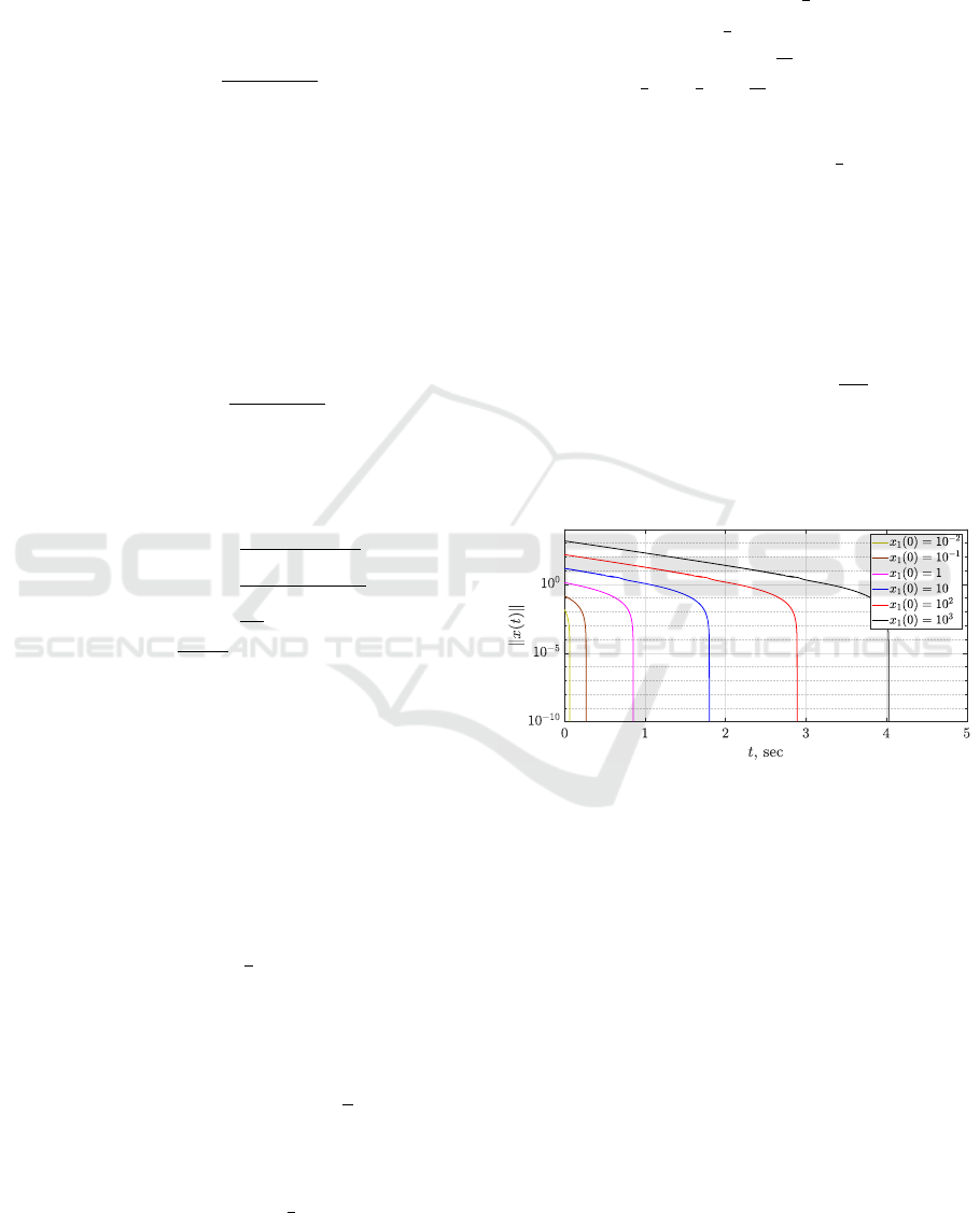
satisfied. Thus, all conditions of Theorem 3 are satis-
fied, and the system is finite-time stable with the fol-
lowing settling time estimate T (x
0
) ≤
3
2
4/3
x
2/3
10
, where
x
10
= x
1
(0). The results of simulation with using
the logarithmic scale are shown in Fig. 1 in order to
demonstrate finite-time convergence rate of the Eu-
clidean norm kxk.
Figure 1: The results of simulation for different initial con-
ditions.
The advantages of the proposed result are based
on the following observations:
• under the condition 2) the finite-time attractive-
ness of the set M is equivalent to finite-time sta-
bility of the origin;
• the condition 1) allows to choose a Lyapunov
function depending only on the variable Ex (e.g.,
V
i
= x
T
E
T
PEx, P > 0 and its nonlinear varia-
tions);
• the terms W
1
and W
2
in the conditions 2) and 4)
become zero along the solutions of the system (1).
In spite of this, these terms are crucial for the
satisfaction of the conditions 2) and 4) in prac-
tice (see, for example, the results of (Ikeda et al.,
2004), (Uezato and Ikeda, 1999) on asymptopic
stability analysis).
Finite-time Stability Analysis for Nonlinear Descriptor Systems
713
If f (x) = 0 only at the origin for x ∈ M then the
following result one can obtain:
Corollary 1. Suppose there exist a continuously dif-
ferentiable function V : R
n
→ R
+
, a continuous func-
tion W : R
n
×R
n−r
→R, functions a,b ∈ K
∞
and real
numbers β ∈ R
+
and σ ∈ [0,1), such that:
1) a(kExk) ≤V (Ex) ≤ b(kExk) for ∀x ∈ R
n
;
2)
˙
V (Ex) +W (x,U
T
f (x)) ≤−βV
σ
(Ex)
for ∀x ∈ R
n
\M ;
3) W(x, 0) ≡ 0 for ∀x ∈ R
n
;
4) {x ∈M : f (x) = 0} ≡{0}.
Then the system (1) is globally finite-time stable and
T (x
0
) ≤
V
1−σ
(Ex
0
)
β(1 −σ)
.
Proof. The proof is straightforward. Accord-
ing to the proof of Theorem 3 the conditions 1) −
3) provide finite-time attractiveness of the set M .
Due to Ex(t) = 0 for ∀t ≥ T
M
(x
0
) =
V
1−σ
(Ex
0
)
β(1−σ)
, then
f (x(t)) = 0 for ∀t ≥ T
M
(x
0
) and by the condition 4)
we have that kxk= 0 for ∀t ≥ T
M
(x
0
), i.e. the system
is finite-time stable with T (x
0
) ≡ T
M
(x
0
).
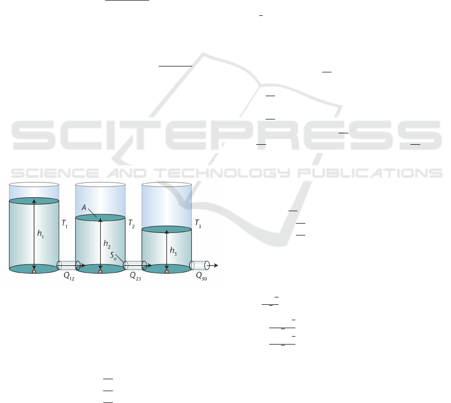
Example 2. Consider the three-tank hydraulic system
(Fig. 2) from (Duro et al., 2008). The system consists
of three cylinders T
1
, T
2
, and T
3
with the same cross-
section A. These cylinders are connected serially to
each other by cross-section S
n
pipes.
Figure 2: Schematic diagram of the three-tank system.
The mathematical model of the plant can be rep-
resented by the following descriptor system:
A
˙
h
1
= −Q
12
,
A
˙
h
2
= Q
12
−Q
23
,
A
˙
h
3
= Q
23
−Q
30
,
Q
12
= S
n
√
2gbh
1
−h
2
e
0.5
,
Q
23
= S
n
√
2gbh
2
−h
3
e
0.5
,
Q
30
= S
n
√
2gbh
3
e
0.5
,
(8)
where h
1
, h
2
and h
3
are the liquid levels in each
tank, their derivatives represent the balance equations;
Q
12
and Q
23
are the flow rates between tanks, Q
30
is the rate of flow exiting the system; g is the ac-
celeration due to gravity; b·e
α
= |·|
α
sign(·). The
system is in the form (1) with E =
AI
3
0
3×3
0
3×3
0
3×3
,
x
T
=
h
1
h
2
h
3
Q
12
Q
23
Q
30
T
. It is easy to
check that the condition 4) of Corollary 1 is satisfied.
Now let us choose the following candidate Lya-
punov function
V (Ex) = |x
1
−x
2
|
1.5
+ |x
2
−x
3
|
1.5
+ |x
3
|
1.5
.
(9)
Recall that by Minkowski inequality for any z
1
,z
2
∈R
and p ≥ 1, the inequality
|z
1
+ z
2
|
p
≤ 2
p−1
(|z
1
|
p
+ |z
2
|
p
)
hold. Applying this inequality one can obtain
1
6
(|x
1
|
1.5
+|x
2
|
1.5
+ |x
3
|
1.5
) ≤V (Ex)
≤ 2
3/2
(|x
1
|
1.5
+ |x
2
|
1.5
+ |x
3
|
1.5
),
i.e., the condition 1) of Corollary 1 is satisfied.
Let
W(x,U
T
f (x)) =
1.5
A
bx
1
−x
2
e
0.5
(2x
4
−2 f
1
(x)−x
5
+ f
2
(x))
+
1.5
A
bx
2
−x
3
e
0.5
( f
1
(x)
−x
4
+2x
5
−2 f
2
(x)−x
6
+ f
3
(x))
+
1.5
A
bx
3
e
0.5
(−x
5
+ f
2
(x) + x
6
− f
3
(x)),
(10)
where f
1
(x) = S
n
√
2gbx
1
−x
2
e
0.5
, f
2
(x) =
S
n
√
2gbx
2
−x
3
e
0.5
and f
3
(x) = S
n
√
2gbx
3
e
0.5
.
According to (8) the function W become zero along
the solutions of the system (the condition 3) of
Corollary 1 hold).
Since
˙
V =
1.5
A
bx
1
−x
2
e
0.5
(−2x
4
+ x
5
)
+
1.5
A
bx
2
−x
3
e
0.5
(x
4
−2x
5
+ x
6
)
+
1.5
A
bx
3
e
0.5
(x
5
−x
6
),
(11)
then, taking into account the equivalence of norms k·
k
1.5
≤ k·k
1
, we obtain
˙
V (Ex) +W (x,U
T
f (x))
=
S
n
√
g
√
2A
"
bx
1
−x
2
e
0.5
bx
2
−x
3
e
0.5
bx
3
e
0.5
#
T
(H + H
T
)
"
bx
1
−x
2
e
0.5
bx
2
−x
3
e
0.5
bx
3
e
0.5
#
≤ −
1.5S
n
√
g
√
2A
(|x
1
−x
2
|+ |x
2
−x
3
|+ |x
3
|)
≤ −
1.5S
n
√
g
√
2A
V
2/3
(Ex),
(12)
where H =
h
−3 3 0
0 −3 3
0 0 −1.5
i
.
Thus, by Corollary 1 the system (8) is finite-time
stable.
Remark 2. Consider the system (1) in the canonical
semi-explicit form
˙x
1
= f
1
(x
1
,x
2
),
0 = f
2
(x
1
,x
2
)
, (13)
ICINCO 2022 - 19th International Conference on Informatics in Control, Automation and Robotics
714

where x =
x
1
x
2
, E =
I
r
0
r×(n−r)
0
(n−r)×r
0
(n−r)×(n−r)
,
f (x) =
f
1
(x
1
,x
2
)
f
2
(x
1
,x
2
)
. Then under the assumption the
function f
2
(x) satisfies the condition that there ex-
ists a continuous function h such that x
2
= h(x
1
) and
h(0) = 0, the system (13) can be reduced to an ODE
˙x
1
= f
1
(x
1
,h(x
1
)),
and finite-time stability analysis methods correspond-
ing to ODEs can be applied (for example, (Bhat
and Bernstein, 2000), (Roxin, 1966), (Bacciotti and
Rosier, 2005), (Moulay and Perruquetti, 2006), etc.).
Note, the representation in the canonical form (13)
and the subsequent transition to ODEs in some cases
can be accompanied by computational complexity
and errors. It is also worth noting that for the sys-
tem in the form (13) the condition 4) of Corollary 1 is
satisfied and the principal conditions are 1) −3).
The next theorem presents the Implicit Lyapunov
Function method (see (Korobov, 1979), (Adamy and
Flemming, 2004)) for finite-time stability analysis of
descriptor systems (1).
Theorem 4. Suppose that there exists a continuous
function
Q: R
+
×R
n
→ R
(V,z) 7→ Q(V,z)
such that
1) Q(V,z) is continuously differentiable ∀z ∈
R
n
\{0} and ∀V ∈ R
+
;
2) for any z ∈ R
n
\{0} there exist V
−
∈ R
+
and
V
+
∈ R
+
:
Q(V
−
,z) < 0 < Q(V
+
,z); (14)
3) for Ω = {(V,z) ∈ R
n+1
: Q(V,z) = 0}
lim
z→0
(V,z)∈Ω
V = 0, lim
V →0
+
(V,z)∈Ω
kzk = 0, lim
kzk→∞
(V,z)∈Ω
V = +∞;
4) the inequality
−∞ <
∂Q(V,z)
∂V
< 0
holds ∀V ∈ R
+
and ∀z ∈ R
n
\{0};
5) the inequality
∂Q(V,z)
∂z
f (x) +W (V,x,U
T
f (x)) ≤βV
σ
∂Q(V,z)
∂V
hold ∀x ∈ R
n
; ∀(V,x) ∈ R
n+1
: Q(V,Ex) = 0, where
z = Ex, W : R
+
× R
n
× R
n−r
→ R is such that
W (V,x,0) ≡ 0, and σ ∈ [0,1), β ∈ R
+
are some con-
stants;
6) {x ∈M : f (x) = 0}≡ {0}.
Then the origin of the system (1) is globally finite-
time stable and
T (x
0
) ≤
V
1−σ
0
β(1 −σ)
,
where V
0
∈ R
+
: Q(V
0
,Ex
0
) = 0.
Proof. The proof follows the same arguments as
one of Corollary 1 and the Implicit Lyapunov Func-
tion method for finite-time stability analysis of ODE
systems (Polyakov et al., 2015, Theorem 4). The
conditions 1), 2), 4) and the implicit function theo-
rem (Courant and John, 2000) imply that the equa-
tion Q(V,z) = 0 implicitly defines a unique function
V : R
n
\{0} → R
+
such that Q(V (z), z) = 0 for all
z ∈ R
n
\{0}. Due to the condition 3) the function V
can be continuously prolonged at the origin by setting
V (0) = 0. In addition, V is radially unbounded and
positive definite. Then there exist functions a,b ∈ K
∞
such that a(kzk) ≤V (z) ≤ b(kzk) (Khalil, 1992), i.e.,
the condition 1) of Corollary 1 is satisfied with z =
Ex.
Since by means of Implicit Function Theorem
(Courant and John, 2000)
˙
V = −
h
∂Q
∂V
i
−1
∂Q
∂z
˙z, then
with z = Ex the condition 5) repeats the conditions 2)
and 3) of Corollary 1. Finally, the condition 6) repeats
the condition 4) of Corollary 1. Thus, all conditions
of Corollary 1 are satisfied and the system (1) is finite-
time stable.
Remark 3. In (Konovalov et al., 2021) a finite-time
homogeneous control is proposed for linear descrip-
tor systems, and the following implicitly defined Lya-
punov function is considered
Q(V,x) = x
T
e
−G
T
d
lnV
X
T
Ee
−G
d
lnV
x −1,
where G
d
∈R
n×n
is an anti-Hurwitz matrix (i.e., −G
d
is Hurwitz); X ∈ R
n×n
is such that X
T
E = E
T
X ≥ 0
and x
T
X
T
Ex = 0 iff Ex = 0. In view of Theorem 4,
the result of (Konovalov et al., 2021) can be revisited
in order to consider an implicitly defined Lyapunov
function in the form
Q(V,x) = z
T
e
−L
T
lnV
Pe
−L lnV
z −1,
P > 0, L is anti-Hurwitz, z = Ex,
(15)
which can be considered as homogeneous generaliza-
tion (see (Konovalov et al., 2021) for more details) of
the quadratic Lyapunov function V (Ex) = x
T
E
T
PEx.
Based on the stability analysis of linear descriptor
systems proposed in (Xu and Lam, 2006), it is ex-
pected that basing on Theorem 4 the choice of a Lya-
punov function in the form (15) may allow one to
obtain more reliable LMI-based stability conditions
and investigate the robustness properties of the con-
trol scheme given in (Konovalov et al., 2021). This is
one of the main directions for future research.
Finite-time Stability Analysis for Nonlinear Descriptor Systems
715

5 CONCLUSION
In this paper, the sufficient conditions of finite-time
stability are proposed for the class of nonlinear de-
scriptor systems. The settling time estimates are ob-
tained. Both, explicit and implicit Lyapunov func-
tion methods are considered. The conditions are suf-
ficiently less restrictive than those proposed in (Chen
and Yang, 2016). The presented finite-time stability
analysis opens a lot of topics for future research. For
example, control and observer design for descriptor
systems based on the proposed stability conditions.
ACKNOWLEDGEMENTS
This work is supported by RSF under grant 22-29-
00344 in ITMO University.
REFERENCES
Adamy, J. and Flemming, A. (2004). Soft variable-structure
controls: a survey. Automatica, 40(11):1821–1844.
Bacciotti, A. and Rosier, L. (2005). Liapunov functions and
stability in control theory. Springer Science & Busi-
ness Media.
Bhat, S. P. and Bernstein, D. S. (2000). Finite-time stability
of continuous autonomous systems. SIAM Journal on
Control and optimization, 38(3):751–766.
Chen, G. and Yang, Y. (2016). Finite time stabilization
of nonlinear singular systems. In 2016 35th Chinese
Control Conference (CCC), pages 516–520. IEEE.
Courant, R. and John, F. (2000). Introduction to calculus
and analysis volume ii/1.
Duro, N., Dormido, R., Vargas, H., Dormido-Canto, S.,
S
´
anchez, J., Farias, G., and Esquembre, F. (2008). An
integrated virtual and remote control lab: The three-
tank system as a case study. Computing in Science &
Engineering, 10(4):50–59.
Hill, D. J. and Mareels, I. M. (1990). Stability theory for dif-
ferential/algebraic systems with application to power
systems. IEEE transactions on circuits and systems,
37(11):1416–1423.
Ikeda, M., Wada, T., and Uezato, E. (2004). Stability
analysis of nonlinear systems via descriptor equations.
IFAC Proceedings Volumes, 37(11):557–562.
Khalil, H. (1992). Nonlinear system. macmillan publishing
company. New York: Wiley, pages 461–483.
Konovalov, D., Zimenko, K., Belov, A., and Wang, H.
(2021). Homogeneity-based finite-time stabilization
of linear descriptor systems. In 2021 60th IEEE Con-
ference on Decision and Control (CDC), pages 3901–
3905. IEEE.
Korobov, V. I. (1979). A solution of the problem of syn-
thesis using a controllability function. In Doklady
Akademii Nauk, volume 248, pages 1051–1055. Rus-
sian Academy of Sciences.
Lopez-Ramirez, F., Efimov, D., Polyakov, A., and Per-
ruquetti, W. (2018). On necessary and sufficient
conditions for fixed-time stability of continuous au-
tonomous systems. In 2018 European control confer-
ence (ECC), pages 197–200. IEEE.
Mo, X., Niu, H., and Lan, Q. (2017). Finite-time stabi-
lization for a class of nonlinear differential-algebraic
systems subject to disturbance. Discrete Dynamics in
Nature and Society, 2017.
Moulay, E. and Perruquetti, W. (2006). Finite time stabil-
ity and stabilization of a class of continuous systems.
Journal of Mathematical analysis and applications,
323(2):1430–1443.
Newcomb, R. (1981). The semistate description of non-
linear time-variable circuits. IEEE Transactions on
Circuits and Systems, 28(1):62–71.
Orlov, Y. (2004). Finite time stability and robust control
synthesis of uncertain switched systems. SIAM Jour-
nal on Control and Optimization, 43(4):1253–1271.
Polyakov, A. (2011). Nonlinear feedback design for fixed-
time stabilization of linear control systems. IEEE
Transactions on Automatic Control, 57(8):2106–
2110.
Polyakov, A., Efimov, D., and Perruquetti, W. (2015).
Finite-time and fixed-time stabilization: Implicit lya-
punov function approach. Automatica, 51:332–340.
Roxin, E. (1966). On finite stability in control sys-
tems. Rendiconti del Circolo Matematico di Palermo,
15(3):273–282.
Sun, L., Feng, G., and Wang, Y. (2014). Finite-time
stabilization and h∞ control for a class of nonlin-
ear hamiltonian descriptor systems with application
to affine nonlinear descriptor systems. Automatica,
50(8):2090–2097.
Uezato, E. and Ikeda, M. (1999). Strict lmi conditions
for stability, robust stabilization, and h/sub/spl in-
fin//control of descriptor systems. In Proceedings of
the 38th IEEE Conference on Decision and Control
(Cat. No. 99CH36304), volume 4, pages 4092–4097.
IEEE.
Wu, H. and Mizukami, K. (1994). Stability and robust sta-
bilization of nonlinear descriptor systems with uncer-
tainties. In Proceedings of 1994 33rd IEEE Confer-
ence on Decision and Control, volume 3, pages 2772–
2777. IEEE.
Xu, S. and Lam, J. (2006). Robust control and filtering of
singular systems, volume 332. Springer.
Yang, C., Sun, J., Zhang, Q., and Ma, X. (2012). Lyapunov
stability and strong passivity analysis for nonlinear de-
scriptor systems. IEEE Transactions on Circuits and
Systems I: Regular Papers, 60(4):1003–1012.
Zheng, C. and Cao, J. (2013). Finite-time synchronization
of singular hybrid coupled networks. Journal of Ap-
plied Mathematics, 2013.
Zimenko, K., Efimov, D., Polyakov, A., and Kremlev, A.
(2021). On necessary and sufficient conditions for out-
put finite-time stability. Automatica, 125:109427.
ICINCO 2022 - 19th International Conference on Informatics in Control, Automation and Robotics
716
