
A Single Motor Driving and Steering Mechanism for a Transformable
Bicycle
Kazuki Sekine
a
and Ikuo Mizuuchi
b
Tokyo University of Agriculture and Technology, 2-24-16 Naka-cho, Koganei-shi, Tokyo 184-8588, Japan
Keywords:
Single Motor, Driving and Steering Mechanism, Self-driving Bicycle, Transforming Mechanism.
Abstract:
This research aims to propose a bicycle capable of transforming into a stable form suitable for autonomous
driving, and achieving both driving and steering with a single motor, using differential drive method. A novel
mechanism of one-motor differential drive using bevel gears and one-way clutches was devised. Then, a
prototype without transforming mechanism was fabricated. An experiment was conducted to demonstrate that
differential drive with a singke motor is possible. In the experiment, the prototype was capable of running
in straight lines and curves with small meandering. Next, to formulate the deceleration of the non-drive side
wheel in the proposed drive mechanism, another series of experiments was conducted. The equation for the
change in wheel rotating speed derived from the results enables accurate estimation of the future position of
the prototype, allowing it to run autonomously in further research.
1 INTRODUCTION
This research aims to transform a bicycle into a stable
form suitable for autonomous driving and to combine
driving and steering with a single motor.
Shared-cycle services are convenient because bi-
cycles can be easily rented, but they require the bi-
cycles to be returned after use. However, the collec-
tion of abandoned bicycles and the redistribution and
rearrangement of excess bicycles at specific return
ports are performed by trucks and other human op-
erators, which reduces the profitability of the shared-
cycle business. Therefore, we consider installing an
autonomous driving function in bicycles to automati-
cally return and relocate bicycles.
In existing research examples of autonomous bi-
cycles, such as Yeh et al.(Ting-Jen Yeh and Tseng.,
2019), two or more motors are used for driving and
steering, which makes the mechanism complex and
causes many failure factors. This makes them un-
suitable for use as shared bicycles, which are used
in large numbers and for long periods. In addition,
autonomous driving in the form of a bicycle requires
some kind of stabilizing mechanisms such as gyro-
scopic mechanism or large landing gears. Even with
those mechanism, there is always a risk of falling.
Also, those mechanisms only make the bicycle heav-
ier and become an obstacle when it is pedaled by a hu-
a
https://orcid.org/0000-0003-3727-8690
b
https://orcid.org/0000-0003-4657-2613
man. So, transforming the bicycle into a stable form
and drive autonomously with a single motor is an ef-
fective way. Naloa et al. (S
´
anchez et al., 2020) de-
veloped an autonomous bicycle with two rear wheels
with variable tread. When the bicycle is driven by hu-
man power, the rear wheels are attached to enable the
bicycle to tilt and turn. When it drives autonomously,
the tread is widened to stabilize. However, the vari-
able tread mechanism requires multiple actuators and
complex mechanisms to deploy, making it impracti-
cal.
Robots driven and steered by a single motor al-
ready exist. Ito et al. (Ito et al., 2019) developed a
single motor robot with passive wheels and propelled
by yaw moment generated by rotating weights. How-
ever, passive wheels limit the ability of robots such as
overcoming steps. So, application to a bicycle is dif-
ficult. Peidr
´
o et al. (Peidr
´
o et al., 2019) developed a
robot with two magnetic or pneumatic adhesion pads
at the bottom of each of the two ends. It can pivot
about different axes by alternately releasing or attach-
ing these pads to the floor. Howver, magnetic adhen-
sion is possible only on a ferromagnetic medium, and
pneumatic adhension needs a vacuum pump, which
requires additional energy. Ribas et al. (Ribas et al.,
2007) developed a three-wheeled robot that only front
wheel is connected to motor. The front wheel is pas-
sively steered by the direction of its rotation. How-
ever, the front wheel always faces almost sideways to
the body, which interferes with the straight-line mo-
tion of the robot. Toyoizumi et al. (Toyoizumi et al.,
Sekine, K. and Mizuuchi, I.
A Single Motor Driving and Steering Mechanism for a Transformable Bicycle.
DOI: 10.5220/0011349200003271
In Proceedings of the 19th International Conference on Informatics in Control, Automation and Robotics (ICINCO 2022), pages 531-538
ISBN: 978-989-758-585-2; ISSN: 2184-2809
Copyright
c
2022 by SCITEPRESS – Science and Technology Publications, Lda. All rights reserved
531
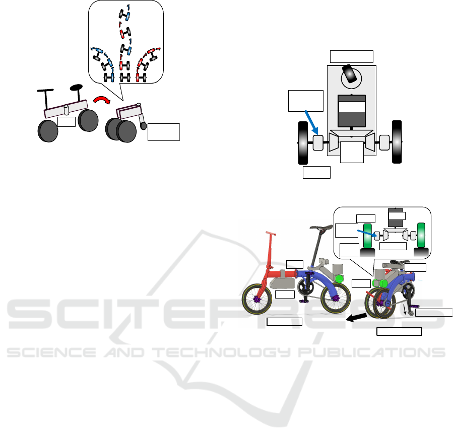
Hinge
Additional
wheel(tilted)
Figure 1: Conceptual diagram.
2010) developed a spherical robot that can generate
both translational and rotational motion with one mo-
tor. However, the spherical shape is unstable and eas-
ily changes its posture when external force is applied,
making it impossible to climb a slope. Zarrouk et
al. (Zarrouk and Fearing, 2015) developed a hexa-
pod robot driven and steered by a single motor. The
robot has two active legs and four passive legs. Cheng
et al. (Cheng et al., 2010) developed a single-motored
soft crawling robot using thermorheological (TR) flu-
ids for modulating the stiffness of its body locally to
change the bending position and direction of it. How-
ever, additional energy is required to heat the fluid,
and the use of tendons for drive makes it difficult
to apply this mechanism to a wheeled robot. Dhar-
mawan et al. (Dharmawan et al., 2017) developed a
four-legged robot driven by a single piezoelectric uni-
morph actuator and capable of moving forward and
turning left or right. However, the driving principle
assumes a legged robot and is difficult to apply to a
wheeled robot. Also, piezoelectric actuators can only
produce very small displacements and require high
voltage, so it can be dangerous.
In this study, we consider using the mechanism of
a folding bicycle to transform the bicycle into a stable
form suitable for autonomous driving, and to combine
driving and steering with a single motor.
2 REALIZATION METHOD
A conceptual diagram of this study is shown in Figure
1. The following conditions are necessary to achieve
the goals of this study.
• Develop a drive mechanism chieving both driving
and steering by a single motor.
• Apply the drive mechanism to a bicycle.
2.1 The Driving and Steering
Mechanism by a Single Motor
14
Motor
Bevel
gears
Wheel
Rear Wheel
One-way
clutch
Figure 2: The proposed drive mechanism.
6
Motor
Bevel gears
Rollers
Additional wheel
One-way
clutch
Battery
Camera
Moving direction
Bicycle mode
Self-driving mode
Roller
Bicycle
tires
Hinge
Figure 3: The 3D modeled transformable bicycle.
In this research, we chose the differential drive
(Dudek and Jenkin, 2010) as a driving method, which
is commonly used as a drive method for two-wheeled
robots. This method uses the difference in rotational
speeds of the left and right wheels to drive and steer
the robot at the same time. In the conventional dif-
ferential drive, each of the left and right wheels has
a motor. In this research, a new mechanism was de-
veloped to realize differential drive with a single mo-
tor. The proposed drive mechanism is shown in Fig-
ure 2. In this mechanism, the motor torque is dis-
tributed to the independent left and right drive shafts
through bevel gears. As a result, the left and right
drive shafts rotate in opposite directions. Wheels are
then attached to the left and right drive shafts via one-
way clutches. The one-way clutch is a mechanism
that transmits torque in only one direction of rotation.
So, for each direction of rotation of the motor, only
one of the left and right wheels rotates in the forward
direction. Therefore, by rotating the motor to forward
and reverse directions in turn, differential drive is pos-
sible with the limitation that the left and right wheels
cannot be driven simultaneously.
ICINCO 2022 - 19th International Conference on Informatics in Control, Automation and Robotics
532
2.2 Application of the Drive Mechanism
to a Bicycle
For the application of the drive mechanism to a bi-
cycle, a folding bicycle that can be folded from the
center of its frame was chosen. Figure 3 shows the
3D modeled transformable bicycle. When folded, the
front and rear wheels of the bicycle face each other
on the right and left sides, so that the robot can easily
stand on its own by adding an wheel to the tail section.
The tread, which is an important factor for the stabil-
ity of a two-wheeled robot, can be easily adjusted by
changing the opening of the hinge used in the folding
process. When the bicycle is pedaled by a human, the
motor drives the rear wheel via a roller. when the bi-
cycle is folded, the front wheel also contacts the other
roller, and both wheels are driven with the differential
drive method. The bicycle drives autonomously using
on-board cameras to recognize their surroundings.
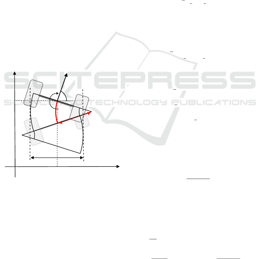
3 MODELING OF DYNAMICS
AND KINEMATICS OF ROBOT
d
l
R
ICC
0
Figure 4: The kinematics of two-wheeled robot.
3.1 Modeling of Kinematics
The kinematics of the robot is modeled by consider-
ing the self-localization using inverse kinematics cal-
culations based on the wheel rotation speeds. First,
consider modeling the dynamics of the robot mov-
ing on a xy-plane as shown in Figure 4. Let q
q
q =
x
c
y
c
θ
c
T
be a vector consisting of the absolute
positionsx
c
, y
c
of the robot and the declination θ
c
from
the x-axis. Given the nonholonomic constraint that
the wheels do not slip or skid, the constraints are im-
posed by the following equation.
˙x
c
sinθ
c
− ˙y
c
cosθ
c
= 0 (1)
Let v be the translation velocity of the robot and ω
be the rotation velocity,
˙
q
q
q is given by the following
equation.
˙
q
q
q =
cosθ
c
0
sinθ
c
0
0 1
v
ω
(2)
In the previous equation, the vector
v ω
T
is given
by :
v
ω
=
r
2
1 1
2
l
−
2
l
˙
θ
l
˙
θ
r
(3)
where r is the wheel radius, l is the tread, and
˙
θ
l
and
˙
θ
r
are the angular velocities of the left and right
wheels, respectively. From Equation (2), (3), the fol-
lowing equation is derived.
˙
q
q
q =
r
2
cosθ
c
cosθ
c
sinθ
c
sinθ
c
2
l
2
l
˙
θ
l
˙
θ
r
(4)
Therefore, the state of the vehicle body q
q
q(t) at a cer-
tain time t is given by the following equation.
x
c
(t) =
r
2
Z
0
t
(
˙
θ
l
+
˙
θ
r
)cosθ
c
(t)dt (5)
y
c
(t) =
r
2
Z
0
t
(
˙
θ
l
+
˙
θ
r
)sinθ
c
(t)dt (6)
θ
c
(t) =
r
l
Z
0
t
(
˙
θ
l
−
˙
θ
r
)d t (7)
During driving, the robot travels in a curve cen-
tered at the Instantaneous Center of Curvature (ICC)
due to the difference in rotational speeds of the left
and right wheels, as shown in Figure 4. In this case,
the radius R of the arc is given by the following equa-
tion.
R =
l(
˙
θ
l
+
˙
θ
r
)
2(
˙
θ
l
−
˙
θ
r
)
(8)
When a robot drive using differential drive by sin-
gle motor, the robot always meandering because it
has a constraint that the both wheels cannot be driven
at the same time. This meandering shortens the dis-
tance the robot can reach. Therefore, in single-motor
diffenrential drive, it is important to minimize it. In
modeling meandering, I defined the meandering rate
D =
d−l
l
. D = 0 when the robot is driving straight.
Here, d is defined as follows.
d =
l
θ
l
− θ
r
2θ
l
− (θ
l
+ θ
r
)cos
r (θ
l
− θ
r
)
2l
(9)
A Single Motor Driving and Steering Mechanism for a Transformable Bicycle
533
3.2 Modeling of Dynamics
In the proposed driving mechanism, the left and right
wheels are driven alternately, so the wheel on the non-
driven side continues to rotate due to inertia and grad-
ually decelerates due to the resistance torque received
from the ground and the drive system. Therefore, ac-
curate estimation of q
q
q at a given time requires model-
ing of the wheel motion. If the rotation angle of the
wheel is θ, the equation of wheel motion is given by
the following equation.
I
¨
θ = τ − τ
v
(
˙
θ) − τ
f
(10)
τ
v
(
˙
θ) = c
v
˙
θ (11)
where I is the moment of inertia including that of the
robot body, τ is the drive torque of the wheel by the
motor, τ
v
(
˙
θ) is the viscous torque, and c
v
is the vis-
cous coefficient. τ
f
is the friction torque. From these
equations, the wheel rotation angle θ is expressed by
the following equation:
θ(t) = Aexp
−
c
v
I
t
−
τ
f
c
v
t + B (12)
where A, B are integral constants. If the initial angle
and angular velocity of the wheel at t = 0 are θ
0
,
˙
θ
0
,
Equation (12) is expressed as follows.
θ(t) = Kexp
−
c
v
I
t
−
τ
f
c
v
t + θ
0
− K
K = −I(c
v
˙
θ
0
+ τ
f
)
(13)
To accurately predict the robot’s future position, each
coefficient in Equation (13) must be estimated by ex-
periment.
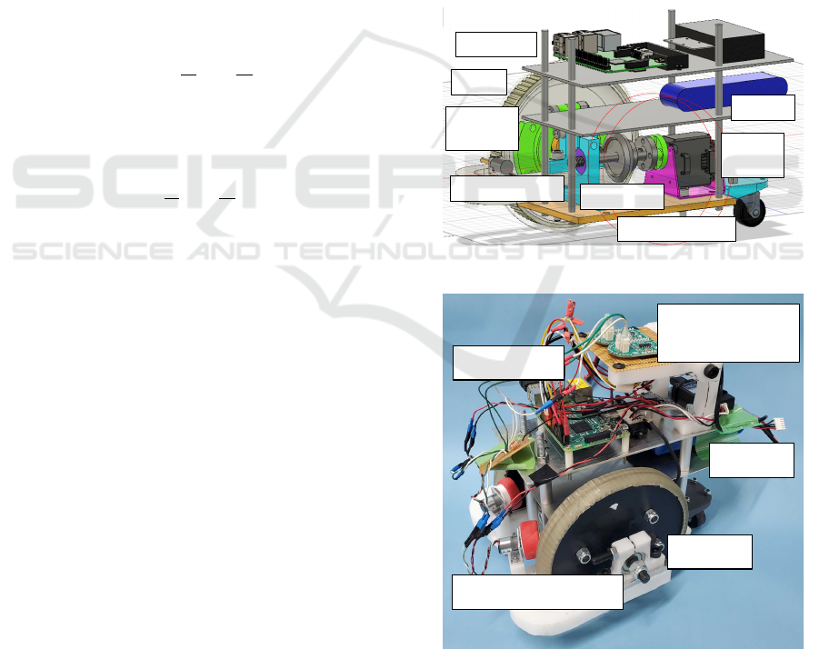
4 DEVELOPMENT OF A ROBOT
FOR DEMONSTRATION OF
DRIVING METHOD
To demonstrate the proposed drive system, a robot
without a folding mechanism was fabricated. Figure
5 shows the structure of the 3D modeled robot and
the developed robot is shown in Figure 6. The robot
is equipped with one Futaba RS406CB serial servo
module. The maximum torque τ
max
is 28.0 kg·cm.
The motor is connected to left and right drive shafts
via bevel gears with a gear ratio of 2:1, as shown in
Figure 7. Therefore, the rotation angles of the wheels
are twice the motor rotation angle. The robot has
two 70 mm radius wheels. The power source is an
11.1V 2100mAh Li-Po battery. The servo module
is connected to an onboard Raspberry Pi 3 Model B
controller via an RSC-U485 USB-RS485 converter.
The robot autonomously drives after receiving com-
mands from an external PC connected to Raspberry
Pi using Wi-Fi. The wheels are 3D printed using
Tough PLA filament and attached to the drive shafts
via Tsubaki BB15-2K-K cam clutches, as shown in
Figure wheel. The friction torque of the cam clutch
is 0.010 Nm. The tires are 3D printed using Form-
labs Elastic 50A Resin. Two Copal RE12D300 Ro-
tary encoders are attached to the left and right wheels
via 15mm radius rollers. Rubber bands are used to
press the rollers against the wheels to keep them from
slipping, as shown in Figure 9. The output signal of
each rotary encoder is counted by the MIKROE-1917
encoder count board and sent to the Raspberry Pi via
SPI communication. Inverse kinematics calculations
are performed to estimate the q of the robot at a given
time based on the angle time series obtained from the
encoders.
One-way
clutch
Wheel
Battery
Controller
Rotary encoder
Additional wheel
Bevel gears
Servo
module
Figure 5: The structure of the 3D modeled robot.
Battery
Wheel
Controller
Rotary encoder
Encoder count
board
Figure 6: The developed robot.
ICINCO 2022 - 19th International Conference on Informatics in Control, Automation and Robotics
534
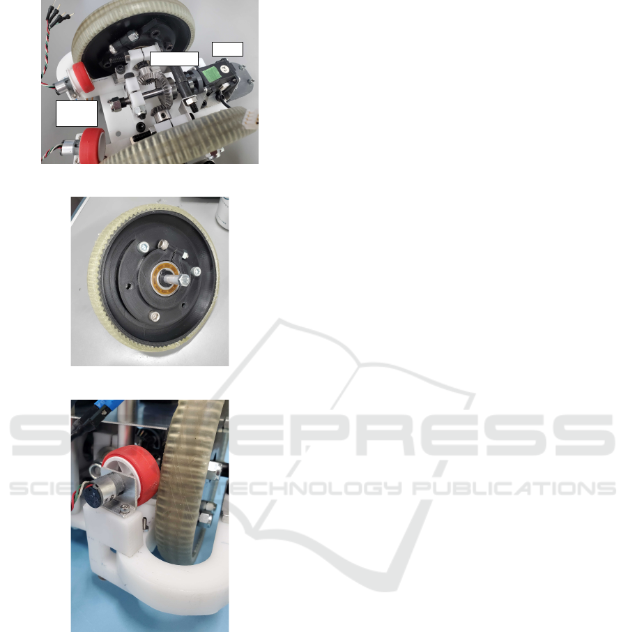
Bevel gears
Rotary
encoders
Motor
Figure 7: The drivetrain of the robot.
Figure 8: The wheel assembly.
Figure 9: The rotary encoder attached to wheel via roller.
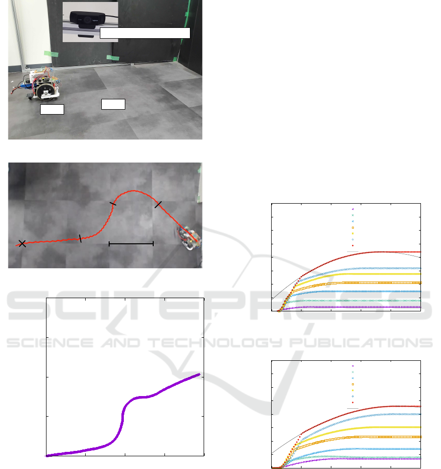
5 EXPERIMENTS
5.1 Demonstration Test of Differential
Drive with a Single Motor
A driving test was conducted to demonstrate the pos-
sibility of driving with differential drive, as shown in
Figure 10. First, the servo module is set to command
mode. In this mode, the target angle and rotating time
can be set using program commands. Then, running
the motor with the target rotation angle and measur-
ing the wheel rotation angle at 10 ms intervals using
rotary encoders.
In this experiment, the robot did the three types of
movements shown below.
• Straight ahead
• Left curve
• Right curve
In the straight movement, the motor alternated be-
tween 20 deg CW and 20 deg CCW rotation at 1 s
intervals. In the left curve movement, the motor alter-
nated between 20 deg CW and k·20 deg CCW rotation
15 times at 1 s intervals. k is a coefficient less than 1,
in this case k = 0.5. This means that the left wheel
has less rotation angle than the right wheel. In the
right curve movement, the motor alternated between
k·20 deg CW and 20 deg CCW rotation 15 times at 1
s intervals. This means that the right wheel has less
rotation angle than the left wheel. Combining these
movements, the robot was made to run in the fol-
lowing order: straight ahead, two curves (left, right),
then straight ahead. The experiment was filmed by a
camera fixed near the ceiling. Then, an open-source
motion analysis software Kinovea was used to extract
the actual trajectory of the robot from the recorded
video and draw it as a line. The trajectory is com-
pared with the trajectory calculated from the rotation
angle measured by rotary encoders. The actual trajec-
tory is shown in Figure 11 and the calculated trajec-
tory is shown in Figure 12 . The calculated trajectory
matched well with the actual trajectory, but a differ-
ence in orientation occurred in the middle of the right
curve. This may be caused by the accumulated er-
rors in the estimated orientation of the robot, due to
the wheels slipping against the floor. The reducing
of the accumulated errors is needed for better self-
localization.
From this experiment, the proposed drive system
was verified by the fact that the machine was able to
move forward while meandering and make left and
right curves.
5.2 Estimation of the Drag Coefficients
of the Robot
In the experiment in Subsection 5.1, the target time
series of the motor rotation angle θ
m
was decided
without considering the robot to reach a specific tar-
get position. To reach a target point, path planning is
needed . For accurate path planning, the estimation of
each drag coefficient c
v
, τ
f
in Equation (13) is needed.
A Single Motor Driving and Steering Mechanism for a Transformable Bicycle
535
Robot
Camera ( near the ceiling )
Floor
Figure 10: Driving test of the robot.
50cm
Start point
Straight
Left curve
Right curve
Straight
Figure 11: The actual trajectory of the robot.
0
0.5
1
1.5
2
0 0.5 1 1.5 2
position y[m]
position x[m]
Figure 12: The calculated trajectory of the robot.
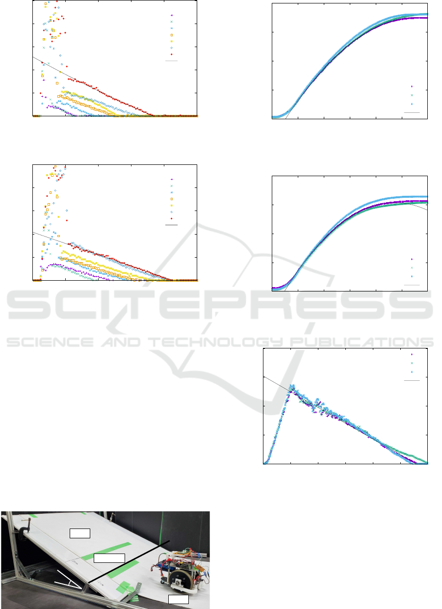
5.2.1 Estimation When Driving on Curves
An experiment was conducted to estimate each drag
coefficient of the robot. First, the robot was put on a
flat floor. Then, one of the wheels is accelerated by
the motor from a standstill to 7 different initial rotat-
ing velocities by setting target angles for the motor in
10 deg increments from 10 deg to 70 deg. Then, the
time variation of wheel rotation angle θ and wheel
rotation velocity
˙
θ is recorded by the rotary encoder
from the moment the motor drive torque τ reaches 0
to the moment the wheel comes to a stop. The result
of experiment is shown in Figure 13-16. The black
lines in Figure 15,16 shows the exponential fitting of
the ’targe angle = 70 deg’ datas, and the black lines
in Figure 13,14 shows the exponential fitting of the
’target angle = 70 deg’ datas.
From these data, the angles and angular velocities
of the left and right wheels θ
L
, θ
R
,
˙
θ
L
,
˙
θ
R
can be ap-
proximated by the following equations.
θ
L
(t) = −7 × 10
3
exp(−3 × 10
−3
t)− 20t + 7 × 10
3
˙
θ
L
(t) = 20exp(−3 × 10
−3
t)− 20
θ
R
(t) = −9 × 10
6
exp(−5 × 10
−5
t)− 700t + 9 × 10
6
˙
θ
R
(t) = 700exp(−7 × 10
−5
t)− 700
(14)
0
50
100
150
200
250
300
350
400
0 20 40 60 80 100
angle[deg]
time[10ms]
target angle = 10 deg
target angle = 20 deg
target angle = 30 deg
target angle = 40 deg
target angle = 50 deg
target angle = 60 deg
target angle = 70 deg
θ
L
=- -7e+03 e
-0.003 t
-2e+01 t+ 7e+03
Figure 13: Time variation of angle of left wheel.
0
50
100
150
200
250
300
350
400
0 20 40 60 80 100
angle[deg]
time[10ms]
target angle = 10 deg
target angle = 20 deg
target angle = 30 deg
target angle = 40 deg
target angle = 50 deg
target angle = 60 deg
target angle = 70 deg
θ
R
=-9e+06 e
-7e-05 t
-7e+02 t+ 9e+06
Figure 14: Time variation of angle of right wheel.
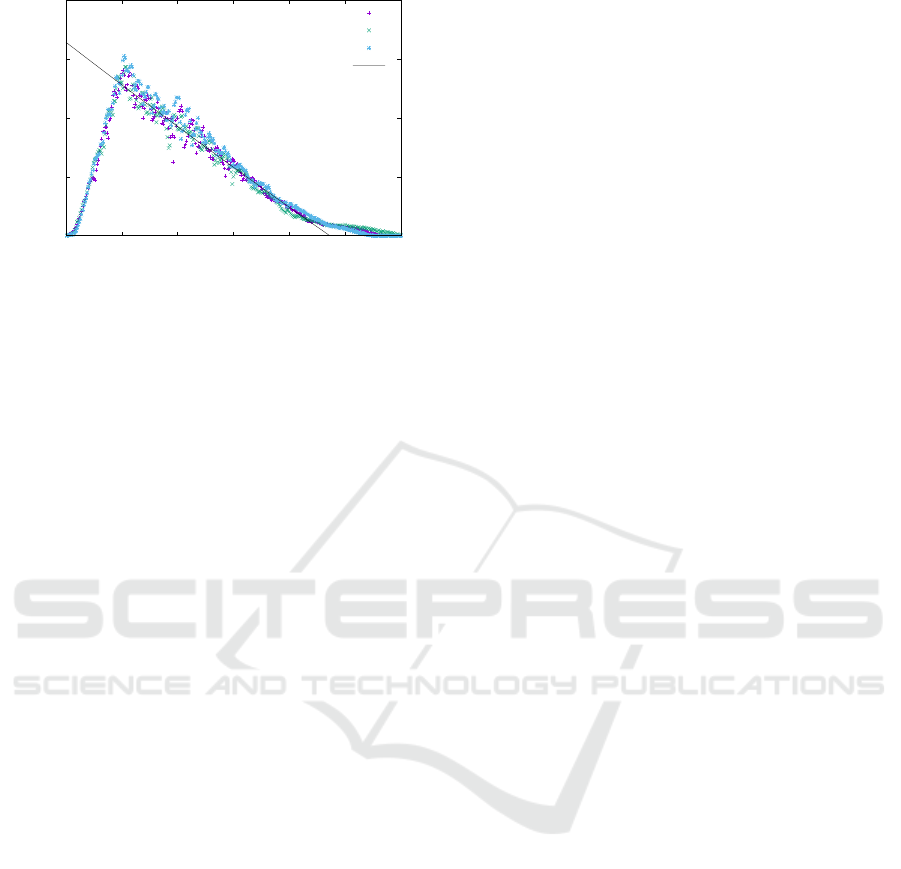
5.2.2 Estimation When Driving Straight
To see if there is a difference, an experiment was con-
ducted in straight-line driving conditions to compare
to the former experiment. A 25 deg slope was set on
the floor, as shown in Figure 17. The robot was held
by hand at a position on the slope, at a height of 10
cm from the ground. When the hand was released,
the robot was accelerated by gravity down the slope
ICINCO 2022 - 19th International Conference on Informatics in Control, Automation and Robotics
536
0
2
4
6
8
10
0 20 40 60 80 100
angular velocity[deg/10ms]
time[10ms]
target angle = 10 deg
target angle = 20 deg
target angle = 30 deg
target angle = 40 deg
target angle = 50 deg
target angle = 60 deg
target angle = 70 deg
θ
.
L
= 2e+01 e
-0.003 t
-2e+01
Figure 15: Time variation of angular velocity of left wheel.
0
2
4
6
8
10
0 20 40 60 80 100
angular velocity[deg/10ms]
time[10ms]
target angle = 10 deg
target angle = 20 deg
target angle = 30 deg
target angle = 40 deg
target angle = 50 deg
target angle = 60 deg
target angle = 70 deg
θ
.
R
= 7e+02 e
-7e-05 t
-7e+02
Figure 16: Time variation of angular velocity of right wheel.
and traveled by inertia on the flat floor. The angle of
rotation of the wheels was measured with rotary en-
coders until the robot came to a stop. The result of
experiment is shown in Figure 18-21. The black lines
in Figure 15,16 shows the exponential fitting of the
’try 1’ data, and the black lines in Figure 13,14 shows
the exponential fitting of the ’try 1’ data. From these
data, θ and
˙
θ can be approximated by the following
equations.
θ
L
(t) = −2 × 10
7
exp(−5 × 10
−5
t)− 100t + 2 × 10
7
˙
θ
L
(t) = 413exp(−1.4 × 10
−4
t)− 397
θ
R
(t) = −4 × 10
5
exp(−4 × 10
−4
t)− 200t + 4 × 10
5
˙
θ
R
(t) = 59exp(−1.2 × 10
−3
t)− 43
(15)
Robot
25deg
Start line
Slope
Figure 17: The slope used in the straight-line experiment.
0
500
1000
1500
2000
0 50 100 150 200 250 300
angle[deg]
time[10ms]
try1
try2
try3
θ
L
=−2e+07 e
−5e−05 t
−1e+03 t+ 2e+07
Figure 18: Time variation of angle of left wheel.
0
500
1000
1500
2000
0 50 100 150 200 250 300
angle[deg]
time[10ms]
try1
try2
try3
θ
R
= −4e+05 e
−0.0004 t
−2e+02 t+ 4e+05
Figure 19: Time variation of angle of right wheel.
0
5
10
15
20
0 50 100 150 200 250 300
angular velocity[deg/10ms]
time[10ms]
try1
try2
try3
θ
.
L
= 1e+03 e
−5e−05 t
−1e+03
Figure 20: Time variation of angular velocity of left wheel.
5.2.3 Discussion
The results of these two experiments follow that the
deceleration of wheel rotations is faster in curved
driving conditions than in straight one. This may
caused by the fact that the rotation angle of the non-
driven wheels were very small when traveling in
curves, causing friction in the direction of yaw rota-
tion of the robot.
A Single Motor Driving and Steering Mechanism for a Transformable Bicycle
537
0
5
10
15
20
0 50 100 150 200 250 300
angular velocity[deg/10ms]
time[10ms]
try1
try2
try3
θ
.
R
= 2e+02 e
−0.0004 t
−2e+02
Figure 21: Time variation of angular velocity of right wheel.
6 CONCLUSIONS
In this study, we proposed a method to transform a
bicycle into a stable form suitable for autonomous
driving and achieve both drive and steer with a single
motor. A prototype without a transforming mecha-
nism was built and tested to demonstrate the proposed
driving method and the driving trajectory estimation
method. We are planning to construct an algorithm
for reaching a goal position and to demonstrate the
algorithm using the prototype. In addition, a regener-
ative mechanism to reduce energy loss due to acceler-
ation and deceleration is planned to be installed in the
prototype. Furthermore, we plan to fabricate an robot
with a transforming mechanism using a folding bicy-
cle and conduct driving tests in an environment that
simulates an actual urban area.
REFERENCES
Cheng, N., Ishigami, G., Hawthorne, S., Chen, H., Hansen,
M., Telleria, M., Playter, R., and Iagnemma, K.
(2010). Design and analysis of a soft mobile
robot composed of multiple thermally activated joints
driven by a single actuator. In 2010 IEEE Interna-
tional Conference on Robotics and Automation, pages
5207–5212.
Dharmawan, A. G., Hariri, H. H., Foong, S., Soh, G. S., and
Wood, K. L. (2017). Steerable miniature legged robot
driven by a single piezoelectric bending unimorph ac-
tuator. In 2017 IEEE International Conference on
Robotics and Automation (ICRA), pages 6008–6013.
Dudek, G. and Jenkin, M. (2010). Computational Princi-
ples of Mobile Robotics. Cambridge University Press,
USA, 2nd edition.
Ito, S., Niwa, K., Sugiura, S., and Morita, R. (2019). An au-
tonomous mobile robot with passive wheels propelled
by a single motor. Robotics and Autonomous Systems,
122:103310.
Peidr
´
o, A., Gallego, J., Pay
´
a, L., Mar
´
ın, J. M., and Reinoso,
´
O. (2019). Trajectory analysis for the masar: A new
modular and single-actuator robot. Robotics, 8:78.
Ribas, L., Mujal, J., Izquierdo, M., and Ramon, E. (2007).
Motion control for a single-motor robot with an un-
dulatory locomotion system. In 2007 Mediterranean
Conference on Control and Automation, pages 1–6.
S
´
anchez, N. C., Pastor, L. A., and Larson, K. (2020).
Autonomous bicycles: A new approach to bicycle-
sharing systems. 2020 IEEE 23rd International Con-
ference on Intelligent Transportation Systems (ITSC),
pages 1–6.
Ting-Jen Yeh, H.-T. L. and Tseng., P.-H. (2019). Balancing
control of a self-driving bicycle. In ICINCO.
Toyoizumi, T., Yonekura, S., Kamimura, A., Tadakuma,
R., and Kawaguchi, Y. (2010). 1-dof spherical
mobile robot that can generate two motions. In
2010 IEEE/RSJ International Conference on Intelli-
gent Robots and Systems, pages 2884–2889.
Zarrouk, D. and Fearing, R. S. (2015). Controlled in-plane
locomotion of a hexapod using a single actuator. IEEE
Transactions on Robotics, 31(1):157–167.
ICINCO 2022 - 19th International Conference on Informatics in Control, Automation and Robotics
538
