
Feedrate Planning for a Delta Parallel Kinematics Numerically
Controlled Machine using NURBS Toolpaths
Gabriel Karasek
a
and Krystian Erwinski
b
Institute of Engineering and Technology, Faculty of Physics Astronomy and Informatics,
Nicolaus Copernicus University, Torun, Poland
Keywords:
Numerical Control, Delta Parallel Kinematics, NURBS, Feedrate Planning.
Abstract:
This paper presents a concept of a computationally efficient feedrate planning algorithm for parallel kinematics
machine in a linear delta configuration. Non-Uniform Rational B-Spline (NURBS) polynomial curve is used
for toolpath definition which provides a smooth trajectory. The feedrate profile is defined as a jerk limited S-
Curve which takes into account limitations stemming from the toolpath curvature and the machine kinematics.
The article presents the outline of the method, structure of the experimental station including the real-time
control system and preliminary experimental results. Further direction of the research is also described. The
proposed method can provide a smooth motion trajectory obtained in real-time with small computational
requirements.
1 INTRODUCTION
In numerical control feedrate is the end effector veloc-
ity tangent to the toolpath. It is the result of combin-
ing the velocities of all of the machine’s axes. Fee-
drate planning is the process of determining a fee-
drate profile that provides a proper value of end ef-
fector feedrate while respecting the machine’s limita-
tions such as maximum velocity, acceleration and jerk
of its axes. These limitations usually stem from lim-
iations of the drive power, drivetrain capabilities or
contouring error.
The feedrate planning problem has been studied
by many researchers for cartesian machines utlizing
optimization algorithms with explicit inclusion of ax-
ial constraints (Mercy et al., 2018; Lu et al., 2018),
tracking error constraints (Zhang et al., 2019) or con-
tour error constraints (Chen and Sun, 2019). Alterna-
tively simplified approaches were proposed using the
feedrate limit function which combines axial limita-
tions of velocity, acceleration and jerk into a single
feedrate limit (Ni et al., 2018b; Ni et al., 2018a; Er-
winski et al., 2022). In the second case the feedrate
profile is usually the widely used jerk-limited s-curve
profile. These feedrate planning methods usually con-
sider cartesian machines sometimes with additional
a
https://orcid.org/0000-0001-8031-8323
b
https://orcid.org/0000-0001-6899-1785
rotary axes in a 5-axis configuration (Li et al., 2021).
Furthermore many of the aforementioned methods
utilize the Non-Uniform B-Spline polynomial curve
as a state-of-the-art way do define the toolpath which
can provide a smooth trajectory compared to typical
G-Code.
The feedrate planning problem for NURBS tool-
paths is more complex for machines with non-
cartesian kinematics which include parallel kinemat-
ics machines. This problem was not investigated pre-
viously as much for these types of machines but is
currently an emerging research topic (Su et al., 2018;
Li et al., 2021). Investigation of feedrate planning
with inclusion of joint/drive limitations is the main
focus of the authors’ current research. The delta par-
allel configuration with linear actuators is the authors’
main focus as such machines can achieve large fee-
drates and therefore high productivity with more stiff-
ness than delta robots with rotary joints. Due to highly
non-linear dependency between joint and end effec-
tor velocities, accelerations and jerks the problem is
much more complex than for cartesian machines. The
inverse kinematics has to be taken into account if ax-
ial constraints are to be considered. Additionally the
authors’ objective is to consider the computational ef-
ficiency and implementation aspects which are impor-
tant if the developed feedrate planning methods are to
be used in practice.
In this paper a computationally efficient method
Karasek, G. and Erwinski, K.
Feedrate Planning for a Delta Parallel Kinematics Numerically Controlled Machine using NURBS Toolpaths.
DOI: 10.5220/0011352900003271
In Proceedings of the 19th International Conference on Informatics in Control, Automation and Robotics (ICINCO 2022), pages 743-749
ISBN: 978-989-758-585-2; ISSN: 2184-2809
Copyright
c
2022 by SCITEPRESS – Science and Technology Publications, Lda. All rights reserved
743
for feedrate planning is presented for a delta paral-
lel kinematics numerically controlled machine. The
jerk limited S-Curve profile is used for feedrate plan-
ning and NURBS curves are used as toolpath defi-
nition. The feedrate planning and NURBS curve in-
terpolation algorithms are described. The experimen-
tal station is described including a description of the
algorithms’ implementation in a real-time Linux op-
erating system. Preliminary experimental results of
the feedrate profile and individual axial velocity, ac-
celeration and jerk profiles and following errors are
presented.
2 NURBS CURVE TOOLPATH
DEFINITION AND
INTERPOLATION
Non-Uniform Rational B-Splines (NURBS) are poly-
nomial spline curves commonly used in computer
graphics but also as definitions of complex shapes
for Computerized Numerically Controlled (CNC) ma-
chines. They are defined in cartesian space using con-
trol points forming a control polygon which roughly
defines the curve’s shape. The shape can be further
influenced by control point weights which pull the
the curve closer to the point if the weight is above
1. NURBS are rational curves which means they can
be used to define most shapes. An additional advan-
tage is the ability to locally influence the shape of the
curve by moving each control point. Furthermore a
curve of a defined degree exhibits continuity of it’s
derivatives if interior knots are not repeated. A cubic
curve has G2 geometric continuity which means that
it’s second derivatives are continuous. This ensures
smoothness of the curve as well as the motion trajec-
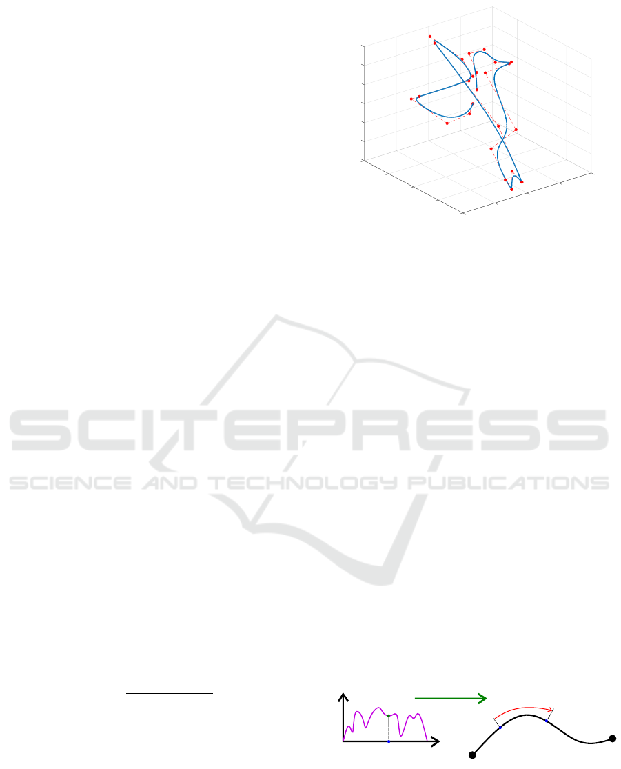
tory of the end effector moving along this curve. An
example of a NURBS curve is shown of Fig.1.
Mathematically NURBS curves are defined as
(Piegl and Tiller, 1996):
C(u) =
n
∑
i=0
N
i,p
(u)w
i
·P
i
n
∑
i=0
N
i,p
(u)w
i
(1)
where: u - curve parameter value, N
i,p
(u) - value of
an elementary polynomial basis function, P
i
- con-
trol point coordinates, w
i
- control point weight. Each
point on the curve is identified by a value of the unit-
less parameter with a value between 0 and 1 which in-
dicate the beginning and end of the curve respectively.
In practice evaluation of the curve is performed us-
ing the numerically stable DeBoor’s algorithm. This
20
100
40
60
50
100
80
Z [mm]
100
50
Y [mm]
0
120
X [mm]
0
140
-50
-50
-100
-100
Figure 1: ”Bird” NURBS toolpath (blue) with marked con-
trol points and polygon (orange).
algorithm is also used to compute curve derivatives
with respect to the curve parameters.
Interpolation is the process of evaluating the tool-
path in constant time intervals to generate points on
the curve. In case of cartesian machines coordinates
of the generated points are the position setpoints of
each machine axis. In case of parallel kinematics ma-
chines the generated coordinates are transformed us-
ing inverse kinematics to generate setpoints for each
joint. In each interpolation step a new value of the
curve parameter u
i+1
is produced corresponding to
the desired arc-length increment and a point on the
NURBS curve C(u
i+1
) is produced using DeBoor’s
algorithm. Arc-length increments ∆s between consec-
utive interpolation points (u
i
,u
i+1
) should be propor-
tional to the desired feedrate F
i
in the current interpo-
lation step. This can be expressed as:
∆s =
Z
u
i+1
u
i
||C
0
(u)||du = V (t
i
) ·∆t (2)
where: C
0
(u) - first derivative of the curve with re-
spect to the curve paramter, V (t
i
) - desired feedrate at
current interpolation time step, ∆t - interpolation time
step. This process is illustrated in Fig.2.
C(u
i
)
Δs = V(
i
) t
t
V
t
i
V(
i
)
FEEDRATE PROFILE
NURBS TOOLPATH
C(u
i+1
)
0
t
end
t
Δ
t
u=0
u=1
Figure 2: Illustration of NURBS interpolation process
based on a polynomial feedrate profile.
The relationship between the curve parameter in-
crement ∆u = u
i+1
−u
i
and arc-length increment ∆S is
non-linear and unique for each curve. This means that
ICINCO 2022 - 19th International Conference on Informatics in Control, Automation and Robotics
744
in each interpolation step this relationship has to be
approximated to satisfy the condition stated in eq.2.
There are several methods of NURBS interpola-
tion such as second and third order Taylor series ap-
proximation, Predictor-Corrector or Feed Correction
Polynomial (Erwinski et al., 2021). In this paper the
second order Runge-Kutta Predictor-Corrector (RK2-
PC) two-step method proposed in (Jia et al., 2017) is
used. In the first step (predictor) a coarse approxima-
tion of the desired curve parameter value is produced:
˜u
i+1
= u
i
+
1
2
(F
1
+ F
2
)∆t (3)
F
1
=
du
dt
=
V (t
i
)
||C
0
(u
i
)||
F
2
=
V (t
i
)
||C
0
(u
i
+ F
1
∆t)||
(4)
In the second step (corrector) a correction increment
∆u
i+1
is determined which modifies the coarse result
˜u
i+1
of the first step. Ideally this should eliminate
the arc-length error so that the following equation is
satisfied:
||C( ˜u
i+1
+ ∆u
i+1
) −C(u
i
)|| = V (t
i
) ·∆t (5)
The end position is rewritten using first order Taylor
expansion and substituted into equation 5. Then both
sides of the obtained formula are squared and after
some manipulations a quadratic equation is obtained:
a ·(∆u
i+1
)
2
+ b ·∆u
i+1
+ c = 0 (6)
a = ||C
0
( ˜u
i+1
)||
2
(7)
b = 2 ·C
0
( ˜u
i+1
) ·(C( ˜u
i+1
) −C(u)) (8)
c = ||C( ˜u
i+1
) −C(u)||
2
−V
2
(t
i
)∆t
2
(9)
The solution to this equation minimizes the interpo-
lation error. The final corrected NURBS parameter
value is thus given by:
u
i+1
= ˜u
i+1
+
−b +
√
a
2
−4a ·b
2a
(10)
It can be seen that in the corrector step the RK2-PC
method uses feedback from a trial interpolation to de-
termine the actual interpolation error. The most com-
monly used 2nd and 3rd order Taylor series approxi-
mations are open-loop methods. They are susceptible
to interpolation error accumulation when large fee-
drates and toolpath curvatures are involved. They also
require computation of higher order NURBS deriva-
tives(Erwinski et al., 2021).
3 DELTA PARALLEL
KINEMATICS
Parallel kinematics is an alternative kinematics con-
figuration, where the end effector is connected with
the drives through two or more independent joints.
Faster feedrate and lower weight of moving system
are the main advantages compared to traditional carte-
sian machines with prismatic joints connected in se-
ries. Also, unlike cartesian machines, there is no ac-
cumulation of positioning error from each axis. All
of axes are moving independently, which means that
the maximum position error is equal to the maximum
error in each axis. Lower weight of individual axes
allows to achieve a lot higher accelerations - up to
300G. (Bouri and Clavel, 2010)
Most popular types of parallel kinematics are ro-
tary delta, mostly used in pick-and-place machines,
and linear delta, which most common applications are
3d printers and robots. This paper will focus on linear
delta machine kinematics. In this type of machines,
linear movements of parallel axes are combined to al-
low movement of end effector in 3 dimensional space.
Main disadvantage of this kinematic configuration is
greater number of mathematical equations, that need
to be solved in order to determine the required joint
setpoints for a desired cartesian position of the end
effector (inverse kinematics).
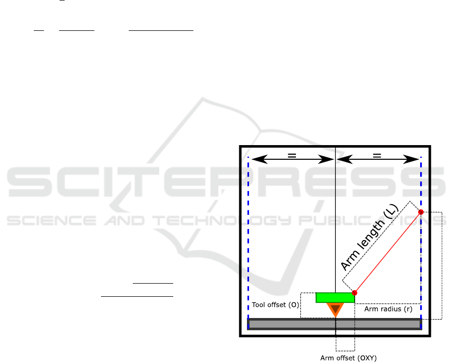
Linear joint position (J
i
)
Figure 3: Effector arm of the delta kinematics machine.
Each of the three vertical linear joints is spread at
an angle of 120 degrees forming an equilateral trian-
gle with the origin in the center equidistant to each of
the vertical joints. As shown in Fig.3, position in X
and Y axes is determined by the size of the effector
plate and arm angle. Z position is dependant on the
height of effector plate above the zero-plane. Usually
it is also required to include end effector or tool off-
set in the Z axis. The inverse kinematics equation for
Feedrate Planning for a Delta Parallel Kinematics Numerically Controlled Machine using NURBS Toolpaths
745
each linear joint is defined by the following formulas:
J
i
= Z +
q
L
2
−(X −r ∗C
i
)
2
−(Y −r ∗S
i
)
2
+ O
(11)
C
i
= cos(α
i
), S
i
= sin(α
i
) (12)
where: J
i
- linear joint positions, X,Y,Z - cartesian
coordinates of end effector position, r - arm radius
(distance between end effector plate and linear joint
carriage in the x,y plane), L - arm length, O - vertical
tool offset, i = A,B,C - linear joint index, α
i
- linear
joint angle (α
A
= 0
◦
,α
B
= 120
◦
,α
C
= 240
◦
)
4 S-CURVE FEEDRATE
PLANNING
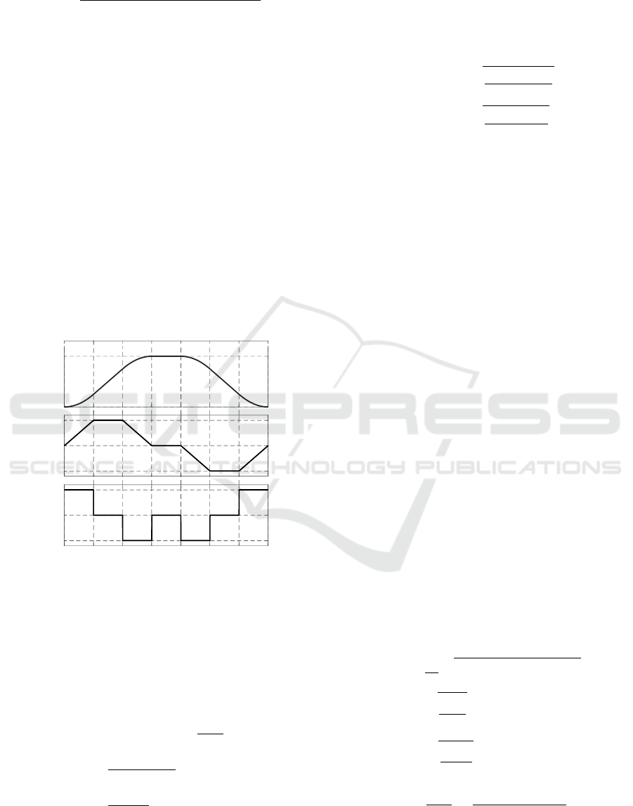
The jerk limited feedrate profile is one of most com-
monly used types of profiling in cnc control systems.
A full profile consist of seven phases which are shown
on fig.4. Depending on the distance between start and
F
start
F
max
F
end
A
max
-A
max
J
max
-J
max
0
0
Feedrate
Acceleration
Jerk
T
1
T
2
T
3
T
6
T
5
T
4
T
7
Figure 4: Example feedrate, acceleration and jerk profiles.
T
1
−T
7
are the durations of each phase of the profile.
end point, start and end velocities (V
start
,V
end
), maxi-
mum feedrate, acceleration and jerk (V
max
,A
max
,J
max
)
the number of phases may be reduced. The algorithm
to determine the duration of each phase is given be-
low.
The duration of each phase of the S-curve profile
is characterized by:
T
1
= T
3
= T
5
= T
7
=
A
max
J
max
(13)
T
2
=
V
max
−V
start
A
max
−T
1
(14)
T
6
=
V
5
−V
6
A
max
(15)
If A
2
max
/J
max
≥V
max
−V
start
the total increase in fee-
drate in phases 1 and 3 is equal or greater than the dif-
ference between start and maximum feedrate. Phase
2 is omitted and acceleration is triangular instead of
trapezoid. Analogously if A
2
max
/J
max
≥ V
max
−V
end
phase 6 is omitted. If phases 2 or 6 are omitted their
duration is 0 and:
T
1
= T
3
=
r
V
max
−V
start
J
max
(16)
T
5
= T
7
=
r
V
max
−V
end
J
max
(17)
After determining the duration of phases 1,2,3,5,6,7
using the formulas given above the distance covered
with the current profile S
tot
is computed. If the dis-
tance is lower than the curve segment arc-length S
seg
for which the profile is generated, phase 4 is added.
The duration of phase 4 with constant maximum fee-
drate of V
max
is T
4
= V
max
/(S
seg
−S
tot
). Otherwise if
the distance S
seg
−S
tot
is negative the maximum fee-
drate has to be lowered and becomes the peak fee-
drate V
peak
. The value of V
peak
has to be determined
numerically. Bisection search is performed between
V
a
= V
max
and V
b
= max(V
start
,V
end
) to find the value
of V
peak
for which the total distance is just below the
segment distance. In each iteration the feedrate pro-
file duration and distance are recomputed with V
peak
instead of V
max
until S
seg
−S
tot
< V
peak
·∆t.
When the NURBS toolpath exhibits areas of sig-
nificant curvature the axial velocities, accelerations
and jerks may vary significantly even if a constant
feedrate is used. This is especially true in case of par-
allel kinematics machines. In order to decrease this
effect a feedrate limit function can be utilized. Such
a function combines axial velocity, acceleration and
jerk limits into a single feedrate limit. Furthermore
chord error limits can also be included. The chord
error is the distance between an arc between two con-
secutive interpolation points and a line between those
points. This approximates the interpolation error due
to discrete interpolation of the curve. The feedrate
limit function (FLF) can be expressed as (Sun et al.,
2019; Zhao et al., 2013):
V
lim
chr
=
2
∆t
q
ρ
2
(u) −(ρ(u) −ε
max
)
2
(18)
V
lim
acc
=
s
A
max
κ(u)
(19)
V
lim
acc
=
3
s
J
max
κ
2
(u)
(20)
κ(u) =
1
ρ(u)
=
||C
0
(u) ×C
00
(u)||
||C
0
(u)||
3
(21)
FLF = min
V
max
,V
lim
chr
,V
lim
acc
,V
lim
acc
(22)
ICINCO 2022 - 19th International Conference on Informatics in Control, Automation and Robotics
746
where: κ - curvature, ρ - curvature radius, ε
max
- max-
imum allowable chord error.
The FLF is used to determine critical points of the
NURBS curve toolpath for which the feedrate has to
be reduced taking into account the maximum allow-
able chord error, feedrate, centripetal acceleration and
jerk. The NURBS curve is evaluated at constant in-
tervals of the u parameter and the value of the FLF is
computed at these points. The array of FLF value is
scanned do determine coarse local minima of the FLF.
A local minimum is a point for which its two neigh-
bouring points have a higher value of the FLF. These
coarse points are then refined using Brent’s method
to find a precise value of the FLF minimum and its
corresponding value of parameter u. The process is
performed for the whole curve and an array of curva-
ture critical points is generated. The S-Curve feedrate
profile is then planned between these critical points
with the FLF values serving as initial and final fee-
drates. Cartesian axis limits are also applied by it-
eratively repeating the interpolation process with the
s-curve segment and verifying if axial constraints are
violated. If that is the case maximum acceleration
and/or jerk maximum values are decreased and the
profile is generated again. This is repeated until all
axial constraints are satisfied. A detailed description
of the algorithm used for a cartesian machine is given
in (Erwinski et al., 2022). The algorithm will be fur-
ther improved to include additional constraints, espe-
cially linear joint velocity, acceleration, constraints.
This will require inclusion of the inverse kinematics
in the feedrate planning process.
5 EXPERIMENTAL STATION
In order to perform real-time control and gather ex-
perimental data a PC-based control system for linear
delta 3D printer was developed. A desktop PC based
controller was used (Intel i3-6100T@3.2GHz, 8GB
RAM) with Linux operating system (DEBIAN 11)
with the kernel patched using the RT-Preempt real-
time patch. This patch enables full kernel preemp-
tion which enables the real-time control processes to
run at the highest priority. LinuxCNC open-source
machine controller software, was installed to utilize
its real-time APIs (HAL and RTAPI). This allowed
to include custom feedrate planning and NURBS in-
terpolation algorithms and run them in the real-time
system. In order to interface the drives EtherCAT
real-time communication bus stack was used based on
the IGH EtherCAT master stack. Nanotec C5E servo-
stepper drives were used with Nema17 stepper motors
equipped with incremental encoders (4000 pulse/rev).
The drives and motors worked in closed loop vec-
tor control mode. All devices were connected via
Ethercat bus. CiA 402 state machine was used. Ad-
equate software driver, that allowed for a cycle time
of 250μs, was developed. Aforementioned driver also
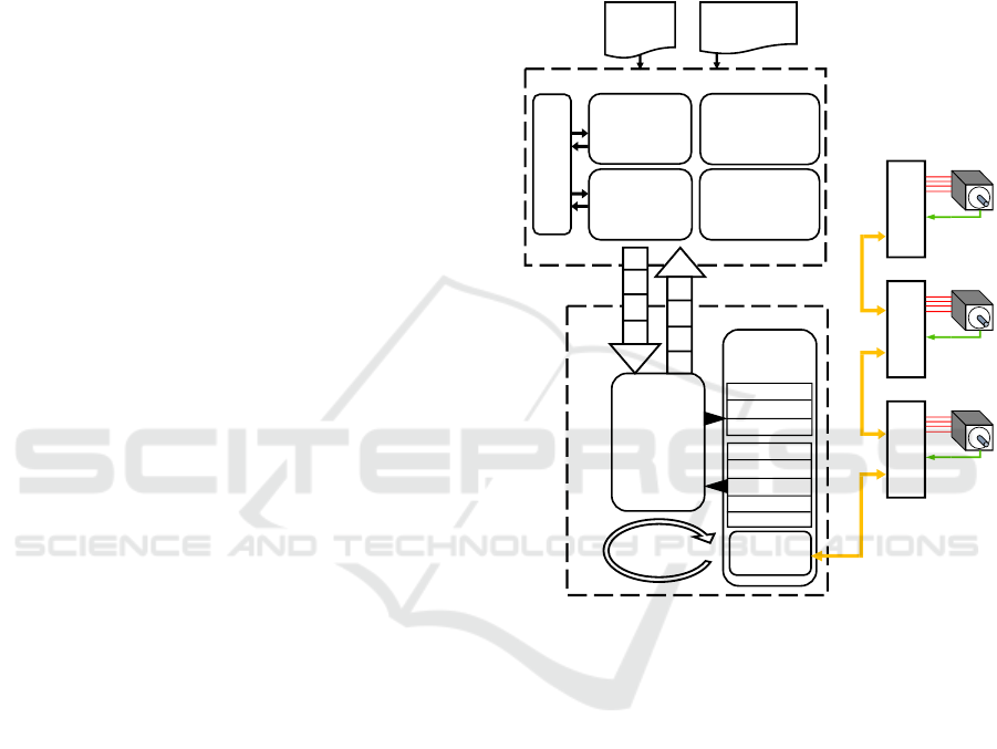
allowed to use HAL API with Nanotec drives. The
block schematic of the experimental station is shown
in Fig.5.
NURBS
TOOLPATH
FEEDRATE
PROFILE
GENERATION
ALGORITHM
PARAMETERS
CONSTRAINTS
MEASUREMENT
DATA AQUISITION,
FILE STORAGE AND
VISUALIZATION
NURBS
TOOLPATH
INTERPOLATION
MODULE
SERVODRIVE
CONTROL
MODULE
CIA402
DEVICE
PROFILE
ETHERCAT
MASTER
STACK
REAL TIME
ETHERNET
DRIVER
REAL-TIME LINUX ENVIRONMENT
SHARED MEMORY
BUFFERS
NON-REAL-TIME PROGRAMS
REAL-TIME
THREAD
(250µs)
CONTROL WORD
POSITION COMMAND
DIGITAL OUTPUTS
STATUS WORD
ACTUAL POSITION
DIGITAL INPUTS
POSITION ERROR
ACTUAL VELOCITY
AUXILIARY
FUNCTIONS
(HOMING, LIMITS,
EMERGENCY STOP)
INVERSE KINEMATICS
TRANSFORMATION
C5E DRIVE
AXIS C
C5E DRIVE
AXIS B
C5E DRIVE
AXIS A
ETHERCAT REAL-TIME BUS
Figure 5: Block schematic of the experimental station’s
control software.
Machine used for testing purposes was all-
aluminum KOSSEL linear delta 3D printer. The Kos-
sel is a modular system for linear delta machines, that
focuses on upgradeability and easy manipulation of
workspace dimensions. This particular machine used
GT2 toothed belts driven directly by the servo-stepper
drives with linear guides (HIWIN MGN12) for in-
creased stiffness. The mechanical parameters of the
machine, are:
• arm length (L): 195mm
• arm radius (r): 65mm
• arm offset (Oxy): 30mm
The picture of the experimental station is shown in
Fig.6.
Feedrate Planning for a Delta Parallel Kinematics Numerically Controlled Machine using NURBS Toolpaths
747
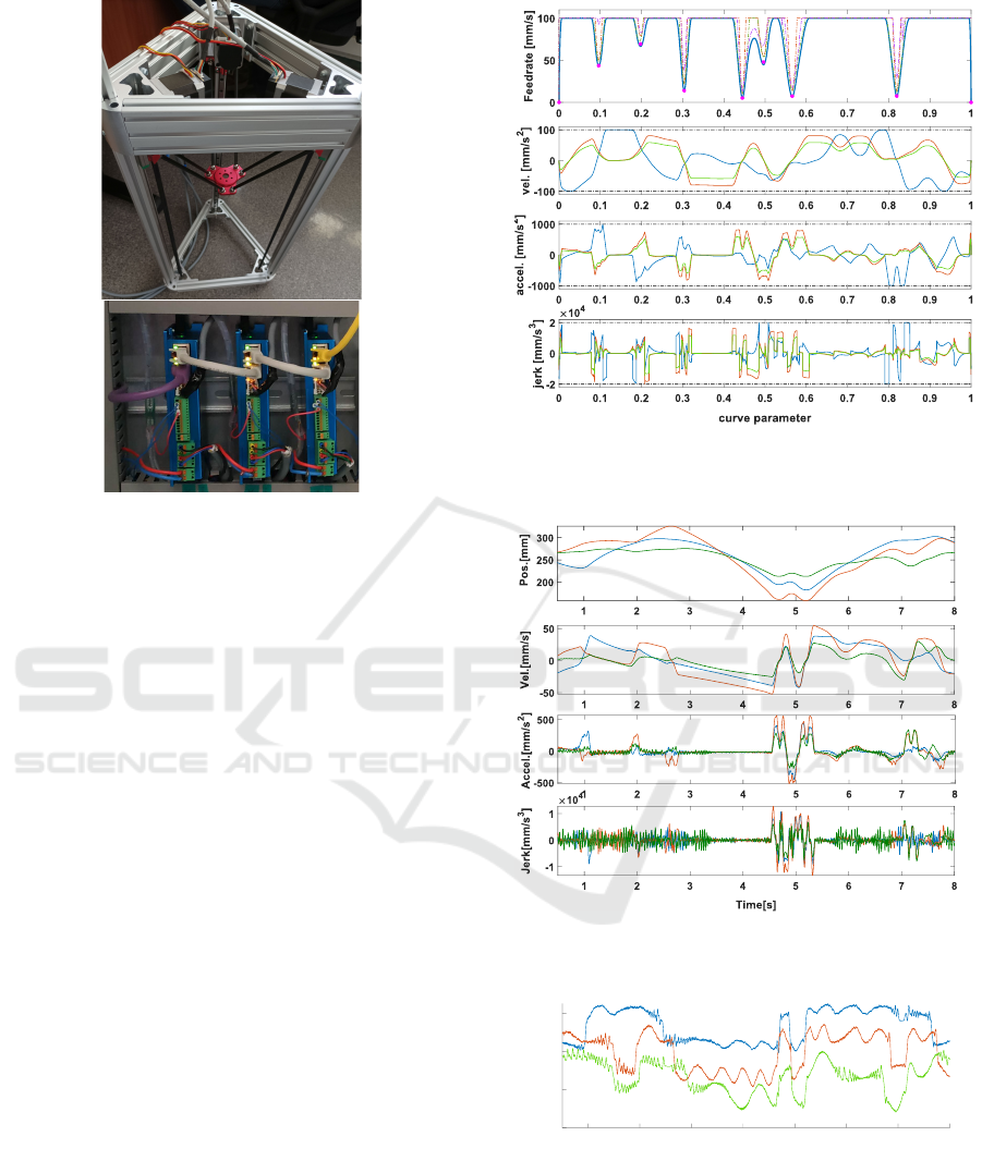
Figure 6: Picture of the Kossel machine used for experi-
mental testing (top) with Nanotec C5E servo-stepper drives
(bottom).
6 EXPERIMENTAL RESULTS
The feedrate profile was generated according to the
feedrate planning algorithm described in Section 4
for the NURBS toolpath presented in Fig.1. Kine-
matic limits were set to V
max
= 100mm/s,A
max
=
1000mm/s
2
,J
max
= 20000mm/s
3
. Maximum chord
error was set to ε = 0.001mm. Figure 7 presents the
generated feedrate profile along with. cartesian axis
velocity, acceleration and jerk. The thick blue line on
the first plot indicates the feedrate profile. The dashed
lines indicate chord error, centripetal acceleration and
jerk components of the Feedrate Limit Function (or-
ange, green and violet respectively). The pink dots
indicate the identified critical points between which
the s-curve feedrate profiles were planned. The sub-
sequent subplots show velocity, acceleration and jerk
in each cartesian axis (blue - X, orange - Y, green -
Z). The dashed black lines indicate the positive and
negative limit of each value.
Fig.8 presents position, velocity, acceleration and
jerk of the linear joints. Fig.9 presents actual follow-
ing error of the linear joints.
It can be seen that the algorithm can limit the
cartesian velocity, acceleration and jerk to their lim-
its despite using the non-linear NURBS toolpath and
an S-Curve feedrate profile. The actual joint lim-
its are not taken into account at this moment. Fur-
ther improvement of the feedrate generation will
lead to inclusion of linear joint limits by applying
Figure 7: Feedrate profile with cartesian axis velocity, ac-
celeration and jerk.
Figure 8: Actual linear joint position, velocity, acceleration
and jerk recorded on the Delta Kossel machine.
1 2 3 4 5 6 7 8
Time[s]
0.15
0.2
0.25
0.3
Following error [mm]
Figure 9: Actual following error of the linear joints
recorded on the Delta Kossel machine.
the inverse kinematics transformation and optimiz-
ing the feedrate profile parameters to meet the lim-
its.Furthermore additional constraints such as follow-
ing and contouring error will be added. The experi-
mental station will also be used for research of posi-
ICINCO 2022 - 19th International Conference on Informatics in Control, Automation and Robotics
748

tioning error and torque ripple compensation meth-
ods using advanced controllers (Tarczewski et al.,
2014),(Tarczewski and Grzesiak, 2009).
In order to verify the computational efficiency of
the algorithm’s implementation in the real-time sys-
tem the feedrate generation process was repeated sev-
eral hundred times and the total computation time was
measured each time. The average computation time
of the whole profile was 99.6ms with maximum and
minimum time equal to 104ms and 97.6ms respec-
tively. The total execution time of the toolpath from
Fig.1 with the feedrate profile from Fig.7 was equal to
8.27s. This means that the proposed method has high
computational effectiveness. The computation time
of feedrate generation algorithm is much shorter than
the toolpath execution time. This means that the sys-
tem with the algorithm has on-line real-time capabili-
ties. Even with the inclusion of additional constraints
such as linear joint constraints the system should still
retain its real-time capabilities.
7 CONCLUSIONS
This paper presents a method for jerk limited fee-
drate planning for Non-Uniform Rational B-Spline
(NURBS) toolpaths in a parallel kinematics machine
in linear delta configuration. The algorithm uses jerk-
limited feedrate planning with limitation of of carte-
sian axes velocity, acceleration and jerk. The pre-
sented experimental results show that the algorithm
can effectively constrain cartesian axis constraints.
Further improvements of the algorithm will constrain
velocity, acceleration and jerk in the linear joints. Fur-
thermore the computation times show that the algo-
rithm is computationally effective and is viable for
real-time implementation. Future research will in-
clude improvement of the algorithm and its extension
with additional constraints.
REFERENCES
Bouri, M. and Clavel, R. (2010). The linear delta: De-
velopments and applications. In ISR 2010 (41st In-
ternational Symposium on Robotics) and ROBOTIK
2010 (6th German Conference on Robotics), pages 1–
8. VDE.
Chen, M. and Sun, Y. (2019). Contour error–bounded para-
metric interpolator with minimum feedrate fluctuation
for five-axis cnc machine tools. Int. J. Adv. Manuf.
Technol., 103(1-4):567–584.
Erwinski, K., Paprocki, M., and Karasek, G. (2021). Com-
parison of nurbs trajectory interpolation algorithms
for high-speed motion control systems. In 2021
IEEE 19th International Power Electronics and Mo-
tion Control Conference (PEMC), pages 527–533.
IEEE.
Erwinski, K., Wawrzak, A., and Paprocki, M. (2022). Real-
time jerk limited feedrate profiling and interpolation
for linear motor multi-axis machines using nurbs tool-
paths. IEEE Transactions on Industrial Informatics
(early access, published online 1.02.2022).
Jia, Z.-Y., Song, D.-N., Ma, J.-W., Hu, G.-Q., and Su, W.-
W. (2017). A nurbs interpolator with constant speed
at feedrate-sensitive regions under drive and contour-
error constraints. Int. J. Mach. Tools Manuf., 116:1–
17.
Li, G., Liu, H., Yue, W., and Xiao, J. (2021). Feedrate
scheduling of a five-axis hybrid robot for milling con-
sidering drive constraints. Int. J. Adv. Manuf. Technol.,
112(11):3117–3136.
Lu, T.-C., Chen, S.-L., and Yang, E. C.-Y. (2018). Near
time-optimal s-curve velocity planning for multiple
line segments under axis constraints. IEEE Trans. Ind.
Electron., 65(12):9582–9592.
Mercy, T., Jacquod, N., Herzog, R., and Pipeleers, G.
(2018). Spline-based trajectory generation for cnc ma-
chines. IEEE Trans. Ind. Electron., 66(8):6098–6107.
Ni, H., Yuan, J., Ji, S., Zhang, C., and Hu, T. (2018a).
Feedrate scheduling of nurbs interpolation based on
a novel jerk-continuous acc/dec algorithm. IEEE Ac-
cess, 6:66403–66417.
Ni, H., Zhang, C., Ji, S., Hu, T., Chen, Q., Liu, Y., and
Wang, G. (2018b). A bidirectional adaptive feedrate
scheduling method of nurbs interpolation based on s-
shaped acc/dec algorithm. IEEE Access, 6:63794–
63812.
Piegl, L. and Tiller, W. (1996). The NURBS book. Springer
Science & Business Media.
Su, T., Cheng, L., Wang, Y., Liang, X., Zheng, J., and
Zhang, H. (2018). Time-optimal trajectory plan-
ning for delta robot based on quintic pythagorean-
hodograph curves. IEEE Access, 6:28530–28539.
Sun, Y., Chen, M., Jia, J., Lee, Y.-S., and Guo, D.
(2019). Jerk-limited feedrate scheduling and opti-
mization for five-axis machining using new piecewise
linear programming approach. Sci. China Technol.
Sci., 62(7):1067–1081.
Tarczewski, T., Grzesiak, L., et al. (2014). Torque ripple
minimization for pmsm using voltage matching cir-
cuit and neural network based adaptive state feedback
control. In 2014 16th European Conference on Power
Electronics and Applications, pages 1–10. IEEE.
Tarczewski, T. and Grzesiak, L. M. (2009). High precision
permanent magnet synchronous servo-drive with lqr
position controller. Electrical Review, 85(8):42–47.
Zhang, Y., Ye, P., Zhao, M., and Zhang, H. (2019). Dy-
namic feedrate optimization for parametric toolpath
with data-based tracking error prediction. Mech. Syst.
Signal Process., 120:221–233.
Zhao, H., Zhu, L., and Ding, H. (2013). A real-time
look-ahead interpolation methodology with curvature-
continuous b-spline transition scheme for cnc machin-
ing of short line segments. Int. J. Mach. Tools Manuf.,
65:88–98.
Feedrate Planning for a Delta Parallel Kinematics Numerically Controlled Machine using NURBS Toolpaths
749
