
Robot Collision Avoidance based on Artificial Potential Field with
Local Attractors
Matteo Melchiorre
a
, Leonardo Sabatino Scimmi
b
, Laura Salamina
c
, Stefano Mauro
d
and Stefano Pastorelli
e
Department of Mechanical and Aerospace Engineering, Politecnico di Torino, C.so Duca degli Abruzzi 24, Turin, Italy
Keywords: Collision Avoidance, Artificial Potential Field, Local Attractors, Motion Planning.
Abstract: This paper presents a novel collision avoidance technique that allows the robot to reach a desired position by
avoiding obstacles passing through preferred regions. The method combines the classical elements of the
artificial potential fields in an original manner by handling local attractors and repulsors. The exact solution,
which is given in a closed form, allows to sculpt a potential field so that local minima related to the local
attractors are prevented and the global minimum is unperturbed. The results show the algorithm applied to
mobile robot navigation and prove the capability of local attractors to influence the robot path.
1 INTRODUCTION
Collision avoidance has long been one of the most
exciting challenges in robotics. It consists in finding
robot commands that satisfy task and spatial
constraints so that the robot reaches a desired
configuration through collision-free motion.
Over the years, several techniques have been
proposed (LaValle, 2006; Siciliano, Sciavicco,
Villani, & Oriolo, 2009). A possible classification can
be made by distinguishing global and local methods
(Abhishek, Schilberg, & Arockia Doss, 2021). Global
methods allow to find a collision-free path from the
initial to the final pose and require prior information
of the environment. They are usually based on
optimization problems, roadmaps or cell
decomposition. On the other hand, local methods
consist of observing the proximity of the robot to
change the path locally in the presence of an obstacle.
Among them it is worth mentioning artificial
potential field (APF), probabilistic roadmaps and
bidirectional RRT.
In particular, APF has been widely investigated
because it is simple to implement and has low
a
https://orcid.org/0000-0002-4409-186X
b
https://orcid.org/0000-0002-0537-2984
c
https://orcid.org/0000-0002-6330-3362
d
https://orcid.org/0000-0001-8395-8297
e
https://orcid.org/0000-0001-7808-8776
computational cost. For this, it performs very well in
dynamic environment, where decisions on the
alternative path must be taken online and a fast robot
response is required.
A first formulation of APF was given by Khatib,
1986. The robot undergoes to virtual forces obtained
from the negative gradient of a potential field, built
considering the target as the attractor, i.e. the global
minimum of the potential, and the obstacles as
repulsors, i.e. confined regions with high potential.
Thereafter, major efforts have been focused on the
local minimum problem, which is the main drawback
of this approach. The most famous examples are the
superquadratic potential function proposed by Volpe
& Khosla, 1990 and the navigation function
introduced by Rimon & Koditschek, 1992 and
extended in Filippidis & Kyriakopoulos, 2011. Other
studies that have been inspired by the drawback of the
artificial potential fields lead to alternative methods,
like the harmonic potential functions (Connolly &
Grupen, 1993), the dynamic window (Fox, Burgard,
& Thrun, 1997), the collision cone (Chakravarthy &
Ghose, 1998) and the attractor dynamics (Haddadin
et al., 2010).
340
Melchiorre, M., Scimmi, L., Salamina, L., Mauro, S. and Pastorelli, S.
Robot Collision Avoidance based on Artificial Potential Field with Local Attractors.
DOI: 10.5220/0011353200003271
In Proceedings of the 19th International Conference on Informatics in Control, Automation and Robotics (ICINCO 2022), pages 340-350
ISBN: 978-989-758-585-2; ISSN: 2184-2809
Copyright
c
2022 by SCITEPRESS – Science and Technology Publications, Lda. All rights reserved

Another branch of the potential field research
moved towards more practical approaches that
consider robot command in terms of a velocity vector
computed from the gradient (Güldner & Utkin, 1996),
or directly obtained in function of the distance from
the obstacle (Mauro et al., 2017; Melchiorre et al.,
2021, 2019; Scimmi et al., 2018, 2019, 2021). This
allows for exact tracking of gradient lines and the
convergence to the goal.
In general, the gradient vector field can be
coupled with additional vector terms to prevent local
minima or to generate convenient paths, that is the
case with tangential fields (De Medio & Oriolo, 1991)
and selective attraction (Murphy, 2000). Another
example is the virtual target approach, that consists of
substituting the global target with a local one around
the object to avoid local minima (Long, 2020; Zou &
Zhu, 2003). Alternatively, the robot goal position can
be temporarily moved or projected to overcome local
minima (Arslan & Koditschek, 2019; Castelnovi,
Sgorbissa, & Zaccaria, 2006; Paromtchik & Nassal,
1995). Other studies consider solving optimization
problem to find the global minimum (Pozna, Troester,
Precup, Tar, & Preitl, 2009).
Plenty of literature works studied how to solve or
improve potential fields built from a single goal and
multiple obstacles but there is a lack of contribute on
techniques to influence trajectory selection in order to
go through specific areas. This can be fundamental
for robot navigation when the obstacle has preferred
approaching directions. For example, socially
acceptable pre-collision criteria suggest that choosing
a certain side when crossing the human path can
improve legibility of robot motion (Qian, Ma, Dai, &
Fang, 2010). Similar aspects arise in human-robot
collaboration, where controlling the robot trajectory
towards predictable regions may result in a more
fluent interaction (Koppenborg, Nickel, Naber,
Lungfiel, & Huelke, 2017).
The importance of finding a simple and effective
solution to deal with obstacles in a controlled manner
motivated the authors of this paper. The original idea
is to introduce local attractors in APF in order to
design the trajectories with a higher precision. Few
authors consider applications of potential fields with
multiple attractors and repulsors. An introduction to
is given in (Beard & McClain, 2003), where, the
possibility to model and combine the potential fields
of each element by using quadratic or exponential
function is discussed. However, (Beard & McClain,
2003) is limited to introducing the concept of multiple
attractors and does not distinguish the roles of the
global and local attractors.
This work investigates the possibility of using
local attractors to make the robot reach the final goal
by avoiding obstacles and passing through attractive
regions. The main aspect that distinguishes this work
from the previous ones is the addition of strategical
attractive points to the one related to the global
minimum. In particular, the attractive points are
modelled as deflections of the potential field, without
being local minima.
2 POTENTIAL FIELD WITH
LOCAL ATTRACTORS
In this section, the problem of artificial potential field
with local attractors is formulated. The avoidance
objectives are: i) to reach a desired position from a
starting configuration; ii) to avoid obstacles choosing
the side of local attractors; iii) to prevent local minima
related to local attractors.
The approach is described in ℝ
2
. The potential
field is modelled combining quadratic and
exponential functions (Beard & McClain, 2003;
Khatib, 1986). Thus, some considerations on the
choice of the attractor intensity are given.
2.1 Problem Formulation
Consider the robot end-effector as a point in the two-
dimensional cartesian space, whose task is to reach
the desired position x
d
from a starting position x
s
. The
desired position can be seen as an attractive potential
field U
d
, which is modelled with the quadratic
function (Khatib, 1986):
𝑈
(
𝒙
)
=
𝜎
‖
𝒙−𝒙
‖
(1)
where 𝜎 is a positive parameter which regulates the
intensity of the quadratic function and x = [x y]
T
represents the generic point in the cartesian space. In
(1), it is written U
d
(x) to exploit the dependency on
x. In general, it is U
d
(x, x
d
, 𝜎) but x
d
is given by the
task and the parameter 𝜎 is supposed to be chosen. To
simplify the reading, hereafter, only the spatial
variable x is exploited, except where otherwise
specified.
Suppose the presence of an obstacle. In general, it
may have any geometry. Sometimes it is convenient
to approximate objects by composing simple shapes,
i.e. spheres, cylinders and planes. Other applications
may need more accurate potential functions to
describe the obstacles. For the discussion, only the
case of the disc in two dimensions, is considered. The
Robot Collision Avoidance based on Artificial Potential Field with Local Attractors
341
reader is referred to the literature for general obstacle
modelling (Khatib, 1986; Ren, Mcisaac, Patel, &
Peters, 2007; Rimon & Koditschek, 1992; Volpe &
Khosla, 1990).
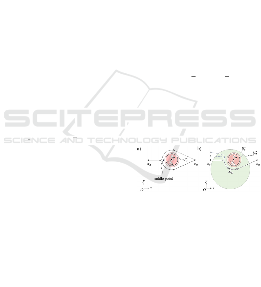
The obstacle is centred in x
o
, with radius R
o
(Figure 1a). It produces a repulsive potential field U
o
,
which is modelled with the exponential function
(Beard & McClain, 2003):
𝑈
(
𝒙
)
=𝛽
𝑒
‖
𝒙𝒙
‖
(2)
where β
o
and γ
o
are the positive parameters that
determine the shape of the gaussian around the
obstacle; in particular, β
o
is the peak value, while γ
o
is
the exponential decay parameter. In Figure 1a, the
outer circle centred in x
o
identifies the active region
U
*
o
, defined as the circle with radius R
*
o
so that the
gradient of U
o
goes to zero outside U
*
o
. The radius R
*
o
can be calculated by solving |∇U
o
| = s
ϵ
, where s
ϵ
is a
small positive value, hereafter named “zero
threshold” (see Appendix A for further details):
𝑅
∗
=−
1
𝛾
𝑊
−
𝑠
𝛽
𝛾
⁄
(3)
If only the goal and the obstacle are considered,
the resulting total potential field U
do
can be written as:
𝑈
(
𝒙
)
=𝑈
(
𝒙
)
+𝑈
(
𝒙
)
=
=
𝜎
‖
𝒙−𝒙
‖
+𝛽
𝑒
‖
𝒙𝒙
‖
(4)
The generic potential field U
do
is shown in Figure 2a.
The control law can be chosen so that the command
vector has the direction of the negative gradient. In
the specific case of Figure 1a, if x
s
, x
o
and x
d
are
aligned, by following the negative gradient the robot
can potentially stuck at the classical saddle point
(Rimon & Koditschek, 1992). This is a limit case. In
fact, in presence of a small perturbation in the y
direction, the robot can potentially trace either the
continue or the dashed path.
In this work, the idea is to introduce an attractive
source x
a
nearby the obstacle, as depicted in Figure
1b. To distinguish the local attractive effect of x
a
from
the global one related to the desired position, x
a
is
called the “local attractor”, while the name “global
attractor” is used to identify x
d
. The local attractor
potential field U
a
is modelled with the negative
exponential function ((Beard & McClain, 2003)):
𝑈
(
𝒙
)
=−𝛼
𝑒
‖
𝒙𝒙
‖
(5)
where α
a
and γ
a
are the positive parameters that
regulate the intensity and the decay of the attractive
effect. In Figure 1b, the circle centred in x
a
identifies
the active region U
*
a
, defined as the circle with radius
R
*
a
so that the gradient of U
a
goes to zero outside U
*
a
.
The parameters α
a
and γ
a
define the active region. For
example, U
*
a
can be extended all around the obstacle
to influence the robot obstacle avoidance on the local
attractor side for a good range of approaching
directions, i.e. for different x
s
(see the path lines in
Figure 1b). Similar to (3), the active region U
*
a
is
determined by solving |∇U
a
| = s
ϵ
:
𝑅
∗
=−
1
𝛾
𝑊
−
𝑠
𝛼
𝛾
⁄
(6)
The total potential field with the obstacle and the
two attractors becomes:
𝑈
(
𝒙
)
=𝑈
(
𝒙
)
+𝑈
(
𝒙
)
+𝑈
(
𝒙
)
=
=
𝜎
‖
𝒙−𝒙
‖
+𝛽
𝑒
‖
𝒙𝒙
‖
−𝛼
𝑒
‖
𝒙𝒙
‖
(7)
A generic potential field U
t
is shown in Figure 2b. The
attractive source x
a
acts bending the potential on its
side. For instance, given γ
a
, a local minimum may
result for high values of the intensity α
a
and the robot
would stop at the equilibrium point close to x
a
.
Anyway, there exist some values of α
a
and γ
a
for
which the total potential field deflates near x
a
without
suffering local minima (Figure 3).
Figure 1: Two-dimensional analysis of the possible robot
paths obtained by following the gradient lines of a quadratic
potential function, with a single obstacle and a local
attractor modelled with the exponential functions. a) In
presence of the obstacle, the robot can potentially follow
either the dashed or the solid lines; in the same figure, the
classical saddle point is shown. b) The robot path is
influenced by the local attractor placed on the obstacle side;
the styles of the lines identify alternative paths related to
different starting positions, i.e. different approaching
directions of the robot towards the obstacle.
ICINCO 2022 - 19th International Conference on Informatics in Control, Automation and Robotics
342
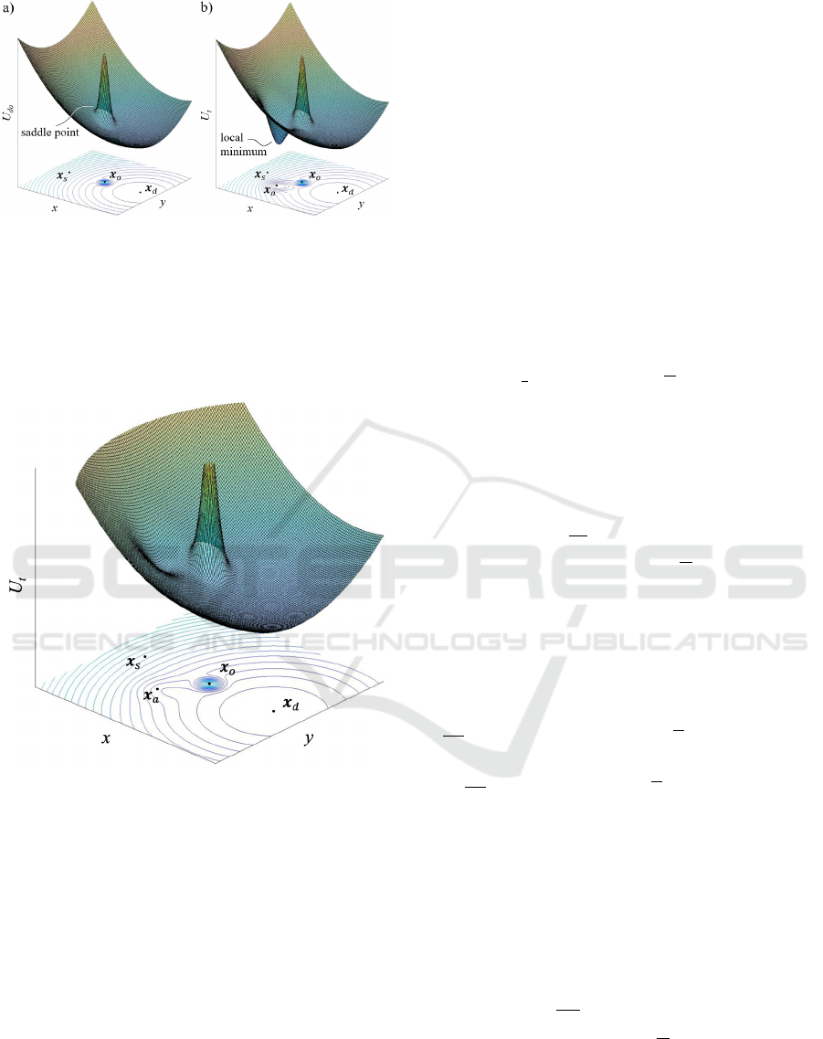
Figure 2: Influence of the exponential repulsive and
attractive potential fields on a quadratic potential field; the
xy plane, in addition to the significant points, contains the
isolines of the potential field. a) Case with a single obstacle;
in the same figure, the classical saddle point is shown. b)
Case with a single obstacle and a local attractor; the high
intensity of the local attractor generates a local minimum,
as indicated by the isolines.
Figure 3: Potential field resulting from a single obstacle and
a local attractor. The intensity of the local attractor is
limited so that the local minimum does not show, as
indicated by the isolines.
2.2 Analysis of the Influence of Local
Attractors
When the obstacle is identified, the attractor x
a
can be
placed near x
o
to affect the collision avoidance path.
It is assumed that x
a
is sufficiently far from the active
region U
*
o
. Without loss of generality the following
relation must hold:
‖
𝒙
−𝒙
‖
>𝑅
∗
+𝜀
̃
(8)
so that the analysis of the local minimum related to
U
a
will simplify. The meaning and the lower bound
of the positive quantity ε͂ will be pointed later.
Moreover, the following assumption which regulates
the size of U
*
a
must be satisfied:
‖
𝒙
−𝒙
‖
𝑅
∗
(9)
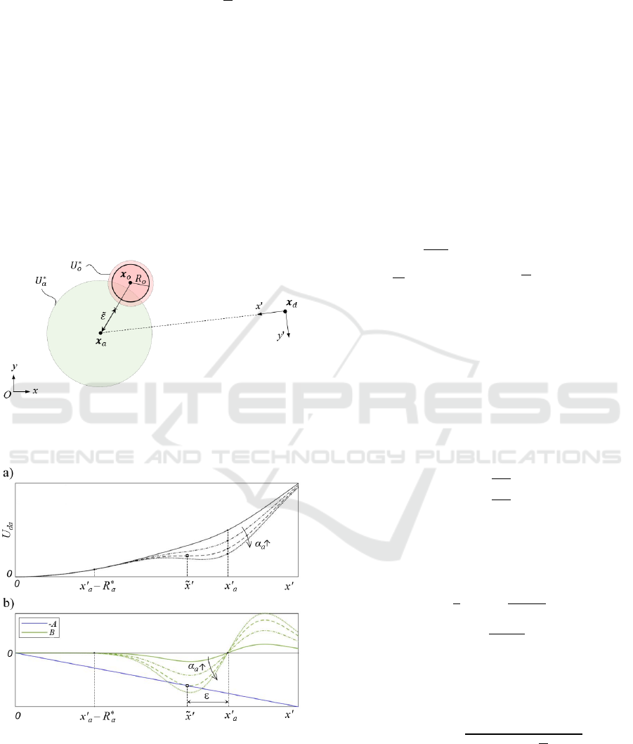
otherwise, the global minimum would be perturbed.
In Figure 4 a generic case which satisfies conditions
(8)-(9) is depicted.
To analyse the influence of α
a
, the local minimum
problem related to x
a
is discussed. This can be dealt
by considering the function U
da
,
defined as the sum of
the two potential fields of the attractors:
𝑈
(
𝒙
)
=𝑈
(
𝒙
)
+𝑈
(
𝒙
)
=
=
𝜎
‖
𝒙−𝒙
‖
−𝛼
𝑒
‖
𝒙𝒙
‖
(10)
In fact, because of assumption (8), the local minimum
will appear in the region where U
o
≃ 0. By studying
the points where the gradient vanishes, the condition
is:
𝜕
𝜕𝒙
𝑈
(
𝒙
)
=
=𝜎
(
𝒙−𝒙
)
+𝛼
𝛾
(
𝒙−𝒙
)
𝑒
‖
𝒙𝒙
‖
=0
(11)
The problem can be further simplified by writing the
system (11) in the auxiliary reference frame O'-x'y'
with origin in O' ≡ x
d
and whose x' axis is aligned
with x
a
(see Figure 4). Thus, by considering
x'
d
= [0 0]
T
and x'
a
= [x'
a
0]
T
the system becomes:
𝜕
𝜕
𝑥
𝑈
(
𝒙
)
=𝜎𝑥
+𝛼
𝛾
(
𝑥
−𝑥
)
𝑒
=0
(12)
𝜕
𝜕𝑦
𝑈
(
𝒙
)
=𝜎𝑦
+𝛼
𝛾
𝑦
𝑒
=0
(13)
where x' = [x' y']
T
is the spatial variable which
identifies a point in the auxiliary reference frame.
Since 𝜎, α
a
and γ
a
are positive, (13) is true only for
y' = 0. This suggests that the local minimum must lie
on the x' axis. Therefore, the problem can be studied
in one dimension. In fact, by considering y' = 0, (12)
reduces to:
𝜕
𝜕𝑥
𝑈
(
𝑥
,0
)
=
=𝜎𝑥
+𝛼
𝛾
(
𝑥
−𝑥
)
𝑒
=0
(14)
Given 𝜎, x'
a
and γ
a
, equation (14) is parametric in α
a
and the number of solutions for x' depend on α
a
. This
can be visualized by plotting the solution in a
Robot Collision Avoidance based on Artificial Potential Field with Local Attractors
343
graphical fashion. By considering:
𝐴=𝜎𝑥
, 𝐵=𝛼
𝛾
(
𝑥
−𝑥
)
𝑒
(15)
the graphical solution is shown in Figure 5b, for fixed
𝜎, x'
a
and γ
a
. In Figure 5a, the resulting potential
U
da
(x', 0) is plotted.
For small values of α
a
, the curves identifying ˗A
and B have only one intersection point at the global
minimum, i.e. in x' = 0. By Increasing the value of α
a
,
the potential starts bending around x' = x'
a
. The value
of α
a
for which U
da
(x', 0) shows a saddle point in
x' = x
͂
', i.e. when the curves ˗A and B become tangent
(dashed line), is then the upper bound ᾶ
a
. For α
a
> ᾶ
a
,
the green and the blue curves intersect in 3 points, i.e.
at the global minimum and at the local stationary
points; in this case the local minimum lies in the
interval 0 < x' < x'
a
.
Figure 4: Generic case with the obstacle and the local
attractor potential functions designed according to the
geometrical constraints.
Figure 5: Analysis of the parametric solution of equation
(14). The different style of the lines refers to different
values of α
a
; the square identify the saddle point related to
the local attractor. a) Potential function U
da
along the x'
axis; the saddle point exists for the dashed line, at x
͂
'. b)
Graphical solution by means of the intermediate variables
(15); the saddle point is represented by the point of
tangency.
The important result is that, given 𝜎, x'
a
and γ
a
, if
α
a
< ᾶ
a
no local stationary points occur. Hereafter, the
saddle point represents the theoretical limit in this
sense: the maximum admissible depression near x'
a
,
i.e. the maximum attraction, is obtained by choosing
an α
a
just below ᾶ
a
.
Notice that, except where otherwise specified, the
saddle point here discussed is the one related to the
local attractor; in fact, the one introduced in Figure 1a
and Figure 2a has a different meaning and it is
identified as the “classical” saddle point.
To find ᾶ
a
, the condition which generates the
saddle is studied. In the saddle point, the first and the
second derivative must vanish. Therefore, (14) must
hold together with the following:
𝜕
𝜕
𝑥
𝑈
(
𝑥
,0
)
=
=𝜎+
1
𝛾
−
(
𝑥
−𝑥
)
𝛼
𝛾
𝑒
=0
(16)
The system of equations (14) and (16) is verified if
(see Appendix B):
(
𝛾
)
𝑥
−
(
2𝑥
𝛾
)
𝑥
+
(
𝑥
𝛾
)
𝑥
−𝑥
=0
(17)
which gives the x' = x
͂
' where the inflection arises (see
Figure 5). The cubic (17) has 3 real solutions for x' if:
𝑥
>
27
4𝛾
(18)
In this case, the meaningful solution is:
𝑥
(
𝑥
,𝛾
)
=
2
3
𝑥
cos
𝜃+4𝜋
3
+1
𝜃(𝑥
,𝛾
)=cos
27
2𝛾
𝑥
−1
(19)
And by substituting (19) in (14) it results:
𝛼
(𝜎, 𝑥
,𝛾
)=
−𝜎𝑥
𝛾
(
𝑥
−𝑥
)
𝑒
(20)
where it is stressed the dependency of ᾶ
a
from 𝜎, x'
a
and γ
a
In general, even if U
a
is centred in x
a
, the sum
with U
d
causes a slight shifting of the inflection in the
ICINCO 2022 - 19th International Conference on Informatics in Control, Automation and Robotics
344
direction of the x' axis, in x
͂
' = [x
͂
' 0]
T
. The shifting can
be quantified considering the distance
||x'
a
˗ x
͂
'|| = x'
a
˗ x
͂
'=𝜀 (see Figure 5). This aspect has
been considered in the assumption (8), so that the
saddle point falls outside U
*
o
.
In particular, two scenarios can be distinguished.
In the first one, the line segment x
a
x
d
does not
intersect U
*
o
; in this case, the stationary point would
fall outside U
*
o
.
The second scenario arises if the line
segment x
a
x
d
crosses U
*
o
: here, if ||x
a
˗ x
o
|| ≤ R
*
o
+ ε the
saddle point of U
da
may overlap with the obstacle;
thus, when considering the total potential U
t
, the
saddle may not exist and the control on the attraction
effect of x
a
is lost. In this case, the main issue is that
the depression which can still manifest within U
*
a
would push the robot towards the obstacle, which is
not advisable. On the other hand, if x
a
x
d
crosses U
*
o
but ||x
a
˗ x
o
|| > R
*
o
+ ε, this will not happen.
From this analysis, the value ε͂ in condition (8) for
the two different scenarios is:
𝜀
̃
=0 𝑖𝑓 𝒙
𝒙
∩𝑈
∗
=0
𝜀
̃
=𝜀 𝑖𝑓 𝒙
𝒙
∩𝑈
∗
≠0
(21)
The steps for sculpting the potential field with local
attractors are summarized by the pseudocode in Table
1.
Table 1: Pseudocode of the APF with local attractors.
1.
define x
s
and x
d
2.
choose 𝜎
3.
identify the obstacle x
o
, R
o
4.
choose γ
o
,
β
o
and s
ϵ
5.
use (3) to find R
*
o
6.
place the local attractor x
a
outside U
*
o
7.
obtain x'
a
= ||x
a
˗ x
d
||, choose γ
a
and verify (18)
8.
calculate ᾶ
a
with (20) and choose α
a
< ᾶ
a
9.
calculate 𝜀
̃
with (21) and verify (8)
10.
find R
*
a
with (6) and verify (9)
11.
obtain 𝑈
as (7)
In the next section, the influence of local attractors
modelled as in Figure 3 is analysed to demonstrate
that this principle can be used to drive the robot on
the side of the local attractor during the obstacle
avoidance manoeuvre, without that the robot get
stuck.
3 APPLICATION
The effectiveness of using local attractors is
investigated considering the case study of a
differential wheeled robot navigating in a structured
environment. The gradient tracking method is chosen
to take full advantage from the potential field
generated with local attractors. This simple and
effective technique produces an exact tracking of the
gradient lines and can be applied to smooth artificial
vector field (Guldner & Utkin, 1995). It consists in
regarding the velocity vector rather than the
acceleration vector as the variable under control.
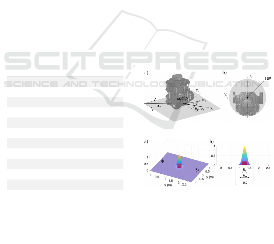
The motion is simulated in Gazebo with the
Turtlebot
®
. Robot commands are given in terms of
linear velocity
𝑣 and angular velocity 𝜔 (Figure 6a).
The angular velocity command is chosen
proportional to the angular error
𝜑 between the
desired direction, identified by the vector v
d
, and the
one of the actual velocity v
r
:
𝜔=𝐾∠𝒗
𝒗
=𝐾𝜑
(22)
where K is the proportional gain and v
d
is chosen as
the negative direction of the gradient:
𝒗
=−∇𝑈
(23)
Figure 6: Gradient tracking (a) and robot size (b).
Figure 7: Obstacle potential field. a) three dimensonal view;
b) lateral view.
As regard the linear velocity command, if v
r
= 0 at the
starting and desired positions, a suitable choice for the
linear velocity magnitude is (Guldner & Utkin, 1995):
𝑣=min
𝑎
𝑡,𝑣
,
(
2𝑎
𝑑
(𝑡)
)
(24)
Robot Collision Avoidance based on Artificial Potential Field with Local Attractors
345
where a
0
is the maximum acceleration, v
0
the
maximum velocity and d
r
(t) = ||x
d
˗ x
r
(t)|| is the
position error.
Different tests are proposed. In each one, a
cylindrical obstacle with radius R
c
= 0.135 m is
placed in the middle between the starting and the
desired robot positions. To consider the robot size
(see Figure 6b), the obstacle potential field is
extended for a wider range, as in (Hossain,
Habibullah, Islam, & Padilla, 2021). In particular, the
parameter γ
o
is chosen so that at a distance
R
o
= (0.135 + 0.105 + s) m the magnitude of the
repulsive gradient is 30% of its maximum value, i.e.
|
∇𝑈
|
𝑅𝑜
=0.3
|
∇𝑈
|
𝑚𝑎𝑥
,
so its value is set as
γ
o
= 80.35
.
The length s is a safety margin and it is set to 0.01 m.
The obstacle and the related potential field obtained
with β
o
= 1 are shown in Figure 7, together with the
mobile robot in one of its starting positions.
Test 1 is made considering the problem
introduced in Figure 1b. The robot starts from
different positions x
s
= [x
s
y
s
]
T
m, with x
s
= 0 and y
s
ranging between 0.05 m and 0.15 m. To influence the
robot path regardless of the approaching direction
against the obstacle, a local attractor is placed on one
side of the obstacle, in x
a
= [0.64 -0.46]
T
m. The
slight displacement 0.05 m representing the lower
limit for y
s
is chosen to exclude the limit case
discussed in Figure 1a and to let the robot choose the
side opposite to x
a
when the local attractor is
removed, as will be seen later.
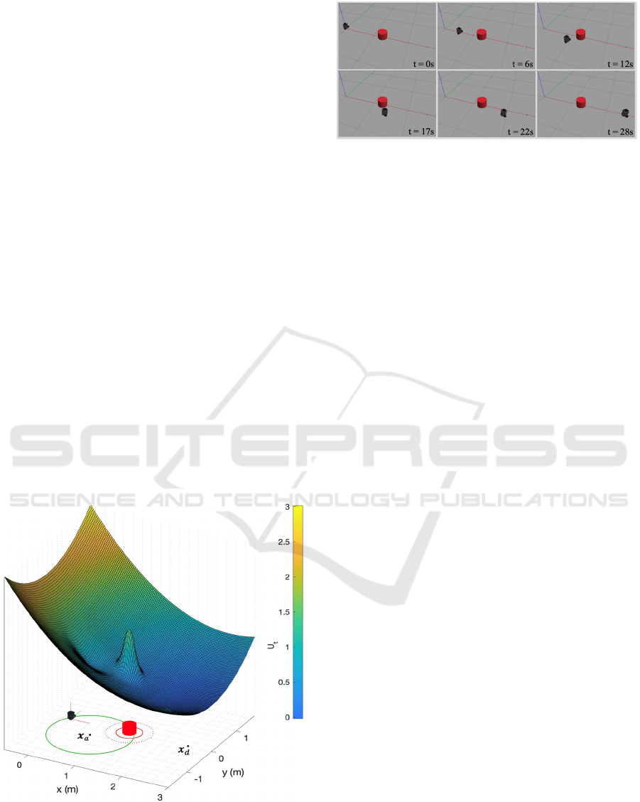
Figure 8: Test layout.
Figure 9: Frames of simulation of Turtlebot in Gazebo.
The global attractor is modelled considering
x
d
= [2.5 0]
T
m, 𝜎 = 0.5, while the local attractor
potential field is obtained with α
a
= 0.266 and
γ
a
= 17.02. The intensity of the local attractor is
chosen as α
a
= 0.8ᾶ
a
, where ᾶ
a
is obtained from (20),
given x'
a
= ||x
a
˗ x
d
||.
The layout of test 1 and the potential field U
t
are
shown in Figure 8. The obstacle position x
o
is known.
The gradient of the potential field is computed in
Matlab and the commands are sent to the robot
through the ROS toolbox, with a control frequency of
30 Hz. The robot motion is characterized by
a
0
= 0.15 m/s
2
, v
0
= 0.1 m/s. and K = 5. The robot
trajectory is obtained through odometry feedback.
Figure 9 shows the frame of the simulation
obtained with x
s
= [0 0.05]
T
m. Results in terms of
path are reported in Figure 10a. The robot is attracted
by x
s
and avoids the obstacle passing on that side. The
effect of the attractor can be seen in Figure 10b, where
the gradient lines of U
t
are depicted.
To evaluate the effectiveness of the potential field
with local attractors, test 2 is performed removing the
local attractor, with x
s
= [0 0.05]
T
m. Results are
shown in Figure 11a and Figure 11b. The robot
follows the gradient and passes the obstacle on the
opposite direction, compared to test 1. Moreover,
because of the greater curvature of the gradient lines
next to the obstacle, the Turtlebot
®
manoeuvre is less
smooth.
The last test, identified as test 3, is carried out to
analyse the effect of the intensity of the local
attractor. Figure 12a shows the different paths
obtained with the same starting position
x
s
= [0 0.05]
T
m and with different values of α
a
. For
α
a
= 0.9ᾶ
a
, the path curve is sharper near the point x
͂
where the saddle would occur for α
a
= ᾶ
a
(see Figure
12b). This is not recommendable, since regions with
high curvature implies sudden change in direction and
may saturate the control resources. However, with
lower values of α
a
the robot can still be guided
towards the side of x
a
, as shown by dashed and dotted
paths in Figure 12a.
ICINCO 2022 - 19th International Conference on Informatics in Control, Automation and Robotics
346
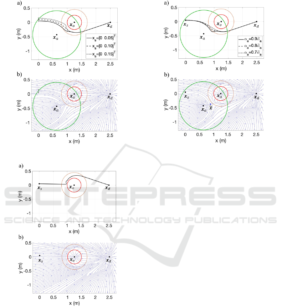
Figure 10: Results of test 1.
Figure 11: Results of test 2.
4 CONCLUSIONS
A new collision avoidance method which aims to
conditionate the robot trajectory by using local
attractors has been presented. The method is inspired
by the previous studies on artificial potential fields
but moves the attention on the role of the attractors
rather than the obstacles.
Figure 12: Results of test 3.
The state of the art of artificial potential fields has
been discussed and a lack of works dealing with local
attractors have been found. Thus, the idea of a new
formula to handle attractors and repulsors coexistence
has been developed with the intention to choose
preferred directions while avoiding collision.
Section 2 describes the theory. The analysis starts
by considering classical exponential functions to
model the potential field for the obstacles and the
attractors. The intuition has been further investigated
by looking for the optimal parameters of the potential
functions to generate the maximum deflection in the
proximity of a local attractor.
In the result section, the algorithm has been tested
on a differential wheeled robot. The robot can avoid
the obstacle choosing the local attractor side, even
considering different approaching directions. Also,
different local attractor intensities have been
considered to show how to obtain smooth trajectories
by regulating the attractive effect.
Future works will focus on the application to real
world scenarios and on the extension to multiple local
attractors or multiple obstacles, with the possibility to
model the potential field related to the obstacles with
different shapes besides disc. Moreover, as the
method is based on potential field, it will be
interesting to extend the theory with dynamic
obstacles and to test how sensory data could affect
collision-free trajectories.
Robot Collision Avoidance based on Artificial Potential Field with Local Attractors
347

REFERENCES
Abhishek, T. S., Schilberg, D., & Arockia Doss, A. S.
(2021). Obstacle Avoidance Algorithms: A Review.
IOP Conference Series: Materials Science and
Engineering, 1012, 012052. https://doi.org/10.1088/17
57-899x/1012/1/012052
Arslan, O., & Koditschek, D. E. (2019). Sensor-based
reactive navigation in unknown convex sphere worlds.
International Journal of Robotics Research, 38(2–3),
196–223. https://doi.org/10.1177/0278364918796267
Beard, R., & McClain, T. (2003). Motion planning using
potential fields. Brigham Young University, BYU
ScholarsArchive, Faculty Publications 1313. Retrieved
from http://www.et.byu.edu/~beard/papers/preprints/
BeardMcLain03-potential.pdf
Castelnovi, M., Sgorbissa, A., & Zaccaria, R. (2006).
Ghost-Goal algorithm for reactive safe navigation in
outdoor environments. In T. Arai et al. (Eds.) (Ed.),
Intelligent Autonomous Systems 9 (pp. 49–56). IOS
Press.
Chakravarthy, A., & Ghose, D. (1998). Obstacle avoidance
in a dynamic environment: A collision cone approach.
IEEE Transactions on Systems, Man, and Cybernetics
Part A:Systems and Humans., 28(5), 562–574.
https://doi.org/10.1109/3468.709600
Connolly, C. I., & Grupen, R. A. (1993). The applications
of harmonic functions to robotics. Journal of Robotics
Systems, 10(7), 931–946. https://doi.org/10.1109/IS
IC.1992.225141
De Medio, C., & Oriolo, G. (1991). Robot Obstacle
Avoidance Using Vortex Fields. Advances in Robot
Kinematics, 227–235. https://doi.org/10.1007/978-3-
7091-4433-6_26
Filippidis, I., & Kyriakopoulos, K. J. (2011). Adjustable
navigation functions for unknown sphere worlds. In
Proceedings of the IEEE Conference on Decision and
Control (pp. 4276–4281). https://doi.org/10.1109/
CDC.2011.6161176
Fox, D., Burgard, W., & Thrun, S. (1997). The dynamic
window approach to collision avoidance. IEEE
Robotics and Automation Magazine, 4(1), 23–33.
https://doi.org/10.1109/100.580977
Guldner, J., & Utkin, V. I. (1995). Sliding Mode Control
for Gradient Tracking and Robot Navigation Using
Artificial Potential Fields. IEEE Transactions on
Robotics and Automation, 11(2), 247–254.
https://doi.org/10.1109/70.370505
Güldner, J., & Utkin, V. I. (1996). Tracking the gradient of
artificial potential fields: Sliding mode control for
mobile robots. International Journal of Control, 63(3),
417–432. https://doi.org/10.1080/00207179608921850
Haddadin, S., Urbanek, H., Parusel, S., Burschka, D.,
Roßmann, J., Albu-Schäffer, A., & Hirzinger, G.
(2010). Real-time reactive motion generation based on
variable attractor dynamics and shaped velocities. In
IEEE/RSJ 2010 International Conference on Intelligent
Robots and Systems (pp. 3109–3116). Taipei.
https://doi.org/10.1109/IROS.2010.5650246
Hossain, T., Habibullah, H., Islam, R., & Padilla, R. V.
(2021). Local path planning for autonomous mobile
robots by integrating modified dynamic-window
approach and improved follow the gap method. Journal
of Field Robotics, (December), 1–16. https://doi.org/
10.1002/rob.22055
Khatib, O. (1986). Real-time obstacle avoidance for
manipulators and mobile robots. International Journal
of Robotics Research, 5(1), 90–98.
Koppenborg, M., Nickel, P., Naber, B., Lungfiel, A., &
Huelke, M. (2017). Effects of movement speed and
predictability in human – robot collaboration. Human
Factors and Ergonomics in Manufacturing & Service
Industries, 27(4), 197–209. https://doi.org/10.1002/
hfm.20703
LaValle, S. M. (2006). Planning algorithms. Planning
Algorithms, 9780521862, 1–826. https://doi.org/10.10
17/CBO9780511546877
Long, Z. (2020). Virtual target point-based obstacle-
avoidance method for manipulator systems in a
cluttered environment. Engineering Optimization,
52(11), 1957–1973. https://doi.org/10.1080/0305215
X.2019.1681986
Mauro, S., Scimmi, L. S., & Pastorelli, S. (2017). Collision
avoidance algorithm for collaborative robotics.
International Journal of Automation Technology,
11(3), 481–489. https://doi.org/10.1007/978-3-319-
61276-8_38
Melchiorre, M., Scimmi, L. S., Mauro, S., & Pastorelli, S.
P. (2021). Vision-based control architecture for
human–robot hand-over applications. Asian Journal of
Control, 23(1), 105–117. https://doi.org/10.1002/asjc.2
480
Melchiorre, M., Scimmi, L. S., Pastorelli, S. P., & Mauro,
S. (2019). Collison Avoidance using Point Cloud Data
Fusion from Multiple Depth Sensors: A Practical
Approach. 2019 23rd International Conference on
Mechatronics Technology, ICMT 2019. https://doi.org/
10.1109/ICMECT.2019.8932143
Murphy, R. R. (2000). Introduction to AI robotics.
Cambridge, Massachusetts: The MIT Press.
Paromtchik, I. E., & Nassal, U. M. (1995). Reactive Motion
Control for an Omnidirectional Mobile Robot. Proc. of
the Third European Control Conference, 5–8.
Pozna, C., Troester, F., Precup, R. E., Tar, J. K., & Preitl,
S. (2009). On the design of an obstacle avoiding
trajectory: Method and simulation. Mathematics and
Computers in Simulation, 79(7), 2211–2226.
https://doi.org/10.1016/j.matcom.2008.12.015
Qian, K., Ma, X., Dai, X., & Fang, F. (2010). Socially
acceptable pre-collision safety strategies for human-
compliant navigation of service robots. Advanced
Robotics, 24(13), 1813–1840. https://doi.org/10.1163/
016918610X527176
Ren, J., Mcisaac, K. A., Patel, R. V, & Peters, T. M. (2007).
A potential field model using generalized sigmoid
functions. Construction,
37(2), 477–484.
Rimon, E., & Koditschek, D. E. (1992). Exact Robot
Navigation using Artificial Potential Functions. IEEE
ICINCO 2022 - 19th International Conference on Informatics in Control, Automation and Robotics
348

Transactions on Robotics and Automation, 8(5), 501–
518. https://doi.org/10.1109/70.163777
Scimmi, L. S., Melchiorre, M., Mauro, S., & Pastorelli, S.
(2018). Multiple collision avoidance between human
limbs and robot links algorithm in collaborative tasks.
ICINCO 2018 - Proceedings of the 15th International
Conference on Informatics in Control, Automation and
Robotics, 2, 291–298. https://doi.org/10.5220/0006852
202910298
Scimmi, L. S., Melchiorre, M., Mauro, S., & Pastorelli, S.
(2019). Experimental Real-Time Setup for Vision
Driven Hand-Over with a Collaborative Robot. 2019
International Conference on Control, Automation and
Diagnosis, ICCAD 2019 - Proceedings. https://doi.org/
10.1109/ICCAD46983.2019.9037961
Scimmi, L. S., Melchiorre, M., Troise, M., Mauro, S., &
Pastorelli, S. (2021). A Practical and Effective Layout
for a Safe Human-Robot Collaborative Assembly Task.
Applied Sciences (Switzerland), 11(4).
Siciliano, B., Sciavicco, L., Villani, L., & Oriolo, G. (2009).
Robotics - Modelling, Planning and Control. Journal of
Chemical Information and Modeling.
Volpe, R., & Khosla, P. (1990). Manipulator control with
superquadratic artificial potential functions: theory and
experiments. IEEE Transactions on Systems, Man and
Cybernetics, 20(6), 1423–1436.
Weisstein, E. (2021). Cubic formula. Retrieved June 7,
2021, from https://mathworld.wolfram.com/Cubic
Formula.html
Zou, X., & Zhu, J. (2003). Virtual local target method for
avoiding local minimum in potential field based robot
navigation. Journal of Zhejiang University Science,
4(3), 264–269.
APPENDIX A
From (2), the gradient of the repulsive potential field
is:
∇𝑈
(
𝒙,𝛽
,𝛾
)
=
𝜕
𝜕𝒙
𝑈
(
𝒙,𝛽
,𝛾
)
=−𝛽
𝛾
(
𝒙−𝒙
)
𝑒
‖
𝒙𝒙
‖
(A1)
More precisely, it is written ∇U
o
(x, β
o
,
γ
o
)
to stress the
dependency on β
o
and γ
o
, that are the design
parameters of the potential field related to the
obstacle. By considering r
o
= ||x ˗ x
o
||, the modulus of
the gradient can be written as:
|
∇𝑈
|(
𝑟
,𝛽
,𝛾
)
=𝛽
𝛾
𝑟
𝑒
(A2)
Outside of the active region the gradient goes to
zero. To quantify this condition, it is assumed that the
gradient magnitude is less than or equal to a small
value s
ϵ
. Thus, by placing |∇U
o
| (r
o
, β
o
, γ
o
) = s
ϵ
in (A2)
and by taking the square, the following relation holds:
−𝛾
𝑟
𝑒
=−
𝑠
𝛽
𝛾
(A3)
which can be written as:
𝑤𝑒
=𝑢
𝑤=−𝛾
𝑟
, 𝑢
=−
𝑠
𝛽
𝛾
(A4)
Equation (A4) can be solved with the Lambert W
function as long as s
ϵ
2
≤ β
o
2
γ
o
/e. Since the latter
condition is easily verified in practice, (A4) has two
real solutions. Without loss of generality, the
meaningful solution corresponds to the lower branch
W
-1
:
𝑤=𝑊
(𝑢
)
(A5)
Equation (A5) solved for r
o
gives (3).
APPENDIX B
From (14):
𝛼
𝛾
𝑒
=
−𝜎𝑥
(
𝑥
−𝑥
)
(B1)
By recognizing this term in (16) and substituting, it
results the cubic (17), which can be written as:
𝑥
−
(
2𝑥
)
𝑥
+
(
𝑥
)
𝑥
−
𝑥
𝛾
=0
(B2)
Equation (B2) can be solved using the cubic formula
(Weisstein, 2021). By considering b
2
= 2x'
a
, b
1
= x'
a
2
and b
0
= ˗x'
a
/γ
a
, the cubic has three real solutions if the
polynomial discriminant D is negative:
𝐷=𝑄
+𝑃
=𝑥
1
4𝛾
−
𝑥
27
<0
𝑄=
=−
𝑃=
=−
+
(B3)
Since x'
a
is positive, condition (B3) translates into
(18). In this case, the three solutions are:
𝑥
=2
−𝑄 cos
𝜃
3
−
𝑏
3
𝑥
=2
−𝑄 cos
𝜃+2𝜋
3
−
𝑏
3
𝑥
=𝑥
=2
−𝑄 cos
𝜃+4𝜋
3
−
𝑏
3
𝜃=cos
𝑃
−𝑄
(B4)
By substituting the three roots in (14), as many
values for α
a
can be found.
Robot Collision Avoidance based on Artificial Potential Field with Local Attractors
349
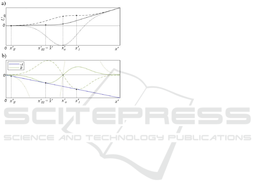
Figure B1 shows the meaning of the three solutions
of a generic case, given 𝜎, x'
a
and γ
a
. The first root x'
I
,
represented by the dashed curve, gives a negative α
a
.
The dotted curve refers to the root x'
II
and to a high
positive value of α
a
, which gives the tangency nearby
the global minimum still producing a local minimum
around x'
a
. The only meaningful solution for the case
study of this paper is then x'
III
, which can be written in
the form (19).
Figure B1: Analysis of the parametric solution of equation
(14). The different style of the lines refers to the 3 values of
α
a
obtained with x
I
, x
II
and x
III
. a) Potential function U
da
along the x' axis. b) Graphical solution by means of the
intermediate variables (15); the squares identify the points
of tangency.
ICINCO 2022 - 19th International Conference on Informatics in Control, Automation and Robotics
350
