
Vision-based Sliding Mode Control with Exponential Reaching Law for
Uncooperative Ground Target Searching and Tracking by Quadcopter
Hamza Bouzerzour
1 a
, Mohamed Guiatni
1 b
, Mustapha Hamerlain
2
and Ahmed Allam
3 c
1
Complex Systems Control and Simulators Laboratory, Ecole Militaire Polytechnique, Algiers, Algeria
2
Centre de D
´
eveloppement des Technologies Avanc
´
ees, Algiers, Algeria
3
Control Process Laboratory, National Polytechnic School, Algiers, Algeria
Keywords:
Quadcopter, Exponential Reaching Law, IBVS, Sliding Mode Control, Ground Target Searching and Tracking.
Abstract:
This paper propose a robust approach based on vision and sliding mode controller for searching and track-
ing an uncooperative and unidentified mobile ground target using a quadcopter UAV (QUAV). The proposed
strategy is an Image-Based Visual Servoing (IBVS) approach using target’s visual data projected in a virtual
camera combined with the information provided by the QUAV’s internal sensors. For an effective visual tar-
get searching, a circular search trajectory is followed, with a high altitude using the Camera Coverage Area
(CCA). A Sliding Mode Controller (SMC) based on Exponential Reaching Law (ERL) is used to ensure the
QUAV control in the presence of external disturbances and measurement uncertainties. Simulation results are
presented to assess the proposer strategy considering different scenarios.
1 INTRODUCTION
Recently, numerous researchers have been interested
in Quadrotor Unmanned Aerial Vehicles (QUAVs)
challenges. The QUAVs are simpler and offer sev-
eral advantages in aspects of maneuverability and
flight stability. They are consequently, used in di-
verse applications, such as transportation (Menouar
et al., 2017), real-time monitoring (Duggal et al.,
2016)(Radiansyah et al., 2017), military reconnais-
sance (Samad et al., 2007) and inspection (Wang
et al., 2022). Mobile Target Tracking is one of the
applications that attract enormous attention, since it
is used in multiple areas, such as, rescue operations
(Cantelli et al., 2013), search and track individu-
als/vehicles (Prabhakaran and Sharma, 2021)(Puri,
2005) and aerial convoys tracking (Ding et al., 2010).
For target tracking, most researchers have mainly
focused on tracking a cooperative target, where its
trajectory is available. Nonetheless, for the uncoop-
erative target it is still a challenging issue. When
the target is occurring suddenly and its information
such as the trajectory and geometrical information is
not accessible, the only available solution to detect
a
https://orcid.org/0000-0002-2218-5777
b
https://orcid.org/0000-0002-5899-6862
c
https://orcid.org/0000-0002-3648-9288
and track it, is the use of the information provided
by an embedded camera. This approach is known
as visual Servoing (VS), which has been the sub-
ject of intensive research since the late 1980s, and it
is classified into two major methods (Janabi-Sharifi
and Marey, 2010). Position-Based Visual Servoing
(PBVS) method, in which, the 3D Cartesian position
of the target is reconstructed from image data and
used to compute the control law. Generally, PBVS
involves more prior knowledge of the camera calibra-
tion parameters and target geometry.
The second method is Image-Based Visual Servoing
(IBVS), where the control law is computed directly in
the 2D image plane. IBVS is widely used due to it
being computation-friendly and to its robustness.
Many researchers have made efforts to address the
IBVS for target tracking (Borshchova and O’Young,
2016)(Pestana et al., 2014). However, the pro-
posed techniques are based on the features Jacobian
(Chaumette and Hutchinson, 2006) under the assump-
tion that the UAV and target performed a smooth
movement variation. But, the use of the features Ja-
cobian may lead to system instability since the QUAV
is an agile system. The solution to overcome this is-
sue is the use of the virtual camera (Fink et al., 2015),
where the image features are projected into a virtual
camera which inherits only the translation and yaw
motion of the real camera.
Bouzerzour, H., Guiatni, M., Hamerlain, M. and Allam, A.
Vision-based Sliding Mode Control with Exponential Reaching Law for Uncooperative Ground Target Searching and Tracking by Quadcopter.
DOI: 10.5220/0011353500003271
In Proceedings of the 19th International Conference on Informatics in Control, Automation and Robotics (ICINCO 2022), pages 555-564
ISBN: 978-989-758-585-2; ISSN: 2184-2809
Copyright
c
2022 by SCITEPRESS – Science and Technology Publications, Lda. All rights reserved
555
Besides the use of the virtual camera, the vision-
based target tracking requires more specific con-
trollers, since the common control algorithms are not
always applicable. Therefore, nowadays many works
are conducted to develop a robust controller to ensure
efficient vision-based target tracking. In (Zhang et al.,
2021), the image moments are defined in the virtual
camera plane and used in a nonlinear model predic-
tive control-based IBVS to track a ground target by
a quadcopter. In (Cao et al., 2017), an IBVS-based
Backstepping controller combined with a nonlinear
trajectory observer is designed to stabilize a quad-
copter above a moving non-cooperative target. Most
of the works have ignored the target searching phase
and have focused only on the development of con-
trollers for the tracking phase, considering that the
target is already detected.
This work proposes a new vision based approach
to control the QUAV for searching and tracking of an
uncooperative and unidentified mobile ground target.
The main contribution is the use of the target’s visual
features expressed in a virtual camera. These fea-
tures are combined with the QUAV’s inertial measure-
ments, camera’s model, as well as the rough informa-
tion of the eventual targets (shape, dimension, maxi-
mum velocity,...etc.). In order to control the QUAV
and to ensure robust autonomous target tracking, a
Sliding Mode Controller (SMC) based on Exponen-
tial Reaching Law (ERL) is designed .
The rest of the paper is organized in seven sec-
tions. Section II presents the problem formula-
tion. Section III presents QUAV’s system description,
modeling and control. Section IV deals with the vi-
sual system modeling while section V focuses on the
target position and velocity estimation using visual
measurements. In section VI, simulation results are
given and discussed.
2 PROBLEM STATEMENT
2.1 Problem Definition
Tracking a ground target by a quadcopter requires the
determination of the quadcopter’s trajectory while the
target remains in its visual field. For more accurate
tracking, the horizontal instantaneous QUAV’s posi-
tion should coincide with the target’s position while
adjusting the QUAV’s altitude to ensure that the tar-
get remains in its FOV.
Therefore, the problem is solved by minimizing the
horizontal position/velocity errors between the quad-
copter and the target. For an uncooperative target-
tracking, it is necessary to establish a flight strategy to
find the target, once the target is found, a vision-based
process should be established to estimate the horizon-
tal position/velocity errors between the target and the
QUAV for which they will be used by the controller.
Hence an adequate controller must be implemented to
handle the proposed flight strategy.
2.2 Proposed Strategy Overview
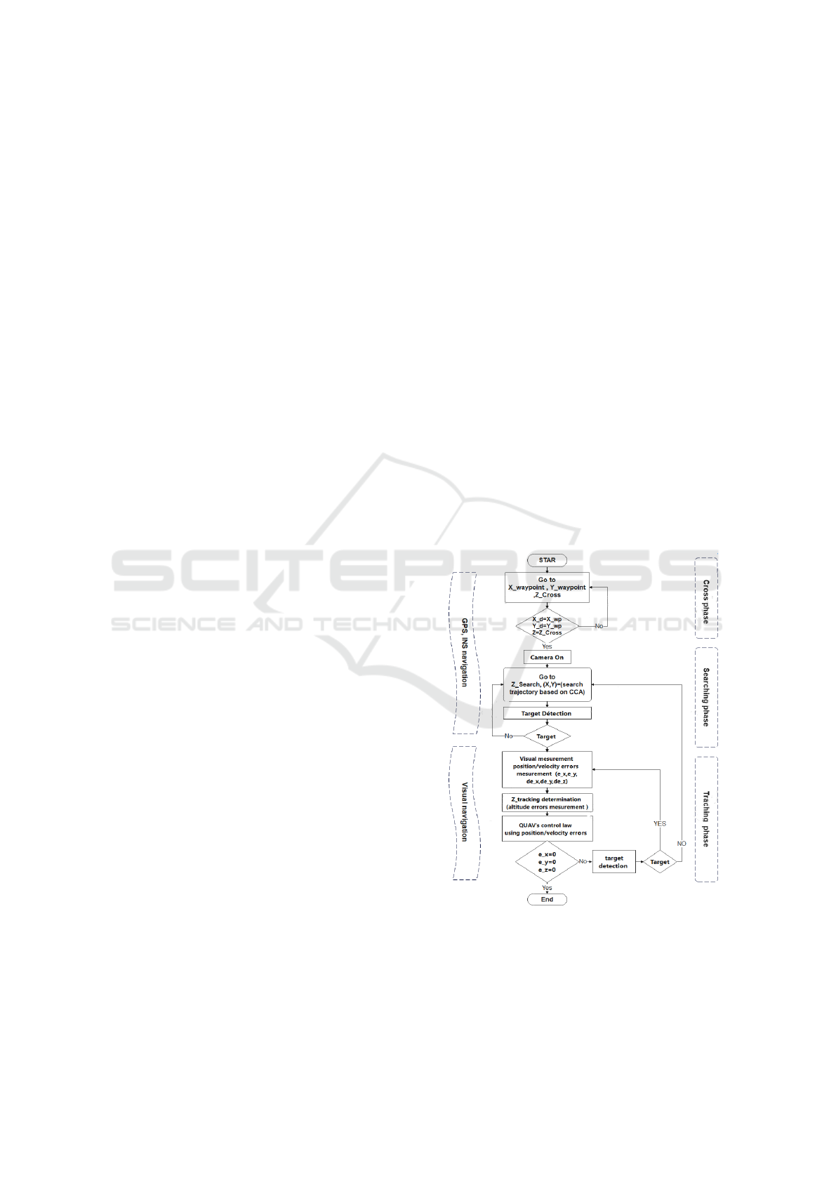
The proposed flight strategy is depicted in Fig. 1,
where the QUAV has at first to reach the area where
the target is supposed to navigate. During this first
phase called cross-phase, the QUAV flies at a low al-
titude to reduce energy consumption and avoid the
wind. Once the QUAV reaches the searching area,
a searching phase is automatically started. For an ef-
fective visual target searching, a circular trajectory is
chosen, with a maximum quadcopter’s altitude. The
said circular trajectory is centered at the start point
and its radius is determined according to the Camera
Coverage Area (CCA). Once the target is detected,
a vision-based tracking process is automatically trig-
gered. During the third phase called the tracking
phase, the QUAV follows the target while tuning its
altitude automatically for optimal target observation.
Figure 1: Flowchart of the proposed strategy.
For the controller, a Sliding Mode Controller
(SMC) based on Exponential Reaching Law (ERL)
is selected. For the first and the second phase, the
control loop uses as a reference the waypoint and the
circular trajectory respectively, which will be com-
ICINCO 2022 - 19th International Conference on Informatics in Control, Automation and Robotics
556
bined with the instantaneous position and altitude of
the QUAV measured by GPS, while for the tracking
phase, the visual measurements are combined with In-
ertial measurement unit (IMU) and the altimeter sen-
sor measurements.
3 QUADCOPTER MODELING
AND CONTROL
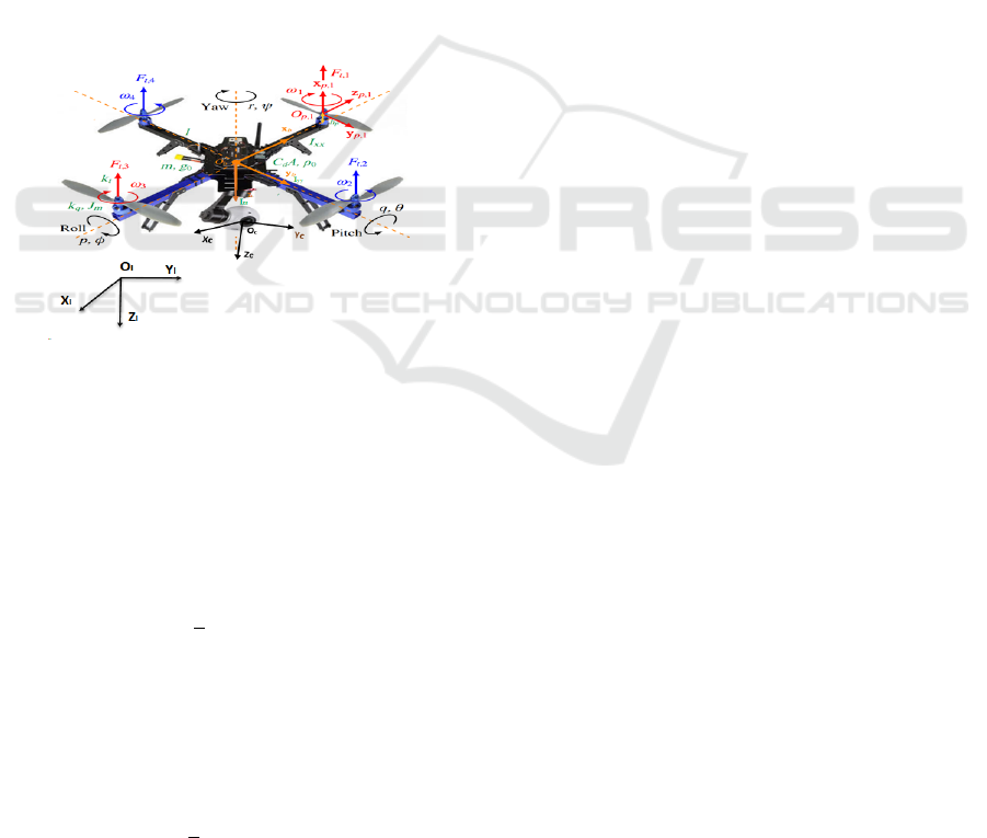
3.1 Quadcopter Modeling
Modeling the concept of visual tracking by a QUAV,
involves the definition of several frames (Fig. 2).
Namely, an inertial fixed frame F
I
= (O
i
,~e
i
x
,~e
i
y
,~e
i
z
),
a body-fixed frame F
B
= (O
b
,~e
b
x
,~e
b
y
,~e
b
z
) attached to
the QUAV mass center, as well as a camera frame
F
C
= (O
c
,~e
c
x
,~e
c
y
,~e
c
z
) attached to the camera’s optical
center.
Figure 2: Quadcopter modeling and frame definition.
The quadcopter consistsof a rigid cross-frame
equipped with four rotors (Fig. 2) and it is assumed
symmetric with respect to the x/y − axis, so that the
center of gravity is located at the center of the struc-
ture, where a monocular camera is fixed.
The QUAV is propelled by four forces
F
i
(i ∈
{
1,2,3,4
}
) generated by the rotation of
the blades mounted on the four rotors.
F
i
=
1
2
ρsC
T
r
2
=bω
2
i
(1)
With ρ and C
T
are the air density and the aerodynamic
thrust coefficients. s/r are the section/radius of the
propeller.
The actuator rotation generates also four drag torques
δ
i
(i ∈
{
1,2, 3,4
}
) which are opposed to the motor
torques
δ
i
=
1
2
ρsC
D
r
2
= dω
2
i
(2)
C
T
is the aerodynamic thrust coefficients.
The QUAV’s attitude is controlled by three
torques U
2
,U
3
,U
4
and the altitude is controlled by the
sum of the four forces U
1
such that :
U
1
U
2
U
3
U
4
=
b b b b
−lb 0 lb 0
0 −lb 0 lb
d −d d −d
ω
2
1
ω
2
2
ω
2
3
ω
2
4
(3)
l is the distance between QUAV’s gravity center and
the rotor.
For the kinematic and dynamic modeling, the QUAV
is considered as 6 − DOF rigid body with mass
m and a constant symmetric inertial matrix J =
diag (I
xx
,I
yy
,I
zz
). Its linear velocity in the F
I
frame
is denoted by V
I
=
˙
ξ = ( ˙x, ˙y, ˙z)
t
and is expressed in
the F
b
frame by the following equation:
v
b
= R
t
V
I
(4)
With v
b
=
u v w
t
. R = R
ψ
R
θ
R
φ
is the rotation
matrix between the F
b
and F
I
frames.
The relation between the derivative of the Eu-
ler angles and the QUAV’s angular velocity Ω =
p q r
t
is given by the following equation:
p
q
r
=
1 0 −S
θ
0 C
φ
S
φ
C
θ
0 −S
φ
C
φ
C
θ
˙
φ
˙
θ
˙
ψ
(5)
Using the Euler Newton formalism, the kinematic
equation is given by:
m
¨
ξ = F
t
− F
d
+ F
g
JΩ = M
f
− M
gp
− M
gb
− M
a
(6)
• F
t
= R.
0 0 −b
ω
2
1
+ ω
2
2
+ ω
2
3
+ ω
2
4
t
is
the total thrust force expressed in F
I
frame;
• F
d
= diag(k
f tx
,k
f ty
,k
f tz
)V
I
is the air drag force
(k
f xi
the drag coefficients);
• F
g
=
0 0 mg
t
is the gravitational force;
• M
a
= diag(k
f ax
,k
f ay
,k
f az
)v
2
b
is aerodynamic
friction torque ( k
f ai
the fiction coefficients);
• M
f
=
U
2
U
3
U
4
t
are the total rolling,
pitching and yawing torques.
• M
gb
and M
gp
are the gyroscopic torques.
Vision-based Sliding Mode Control with Exponential Reaching Law for Uncooperative Ground Target Searching and Tracking by
Quadcopter
557
Using (3) and (6), the QUAV model is given by:
˙p = a
1
qr − a
3
¯
Ω
r
q + a
2
p
2
+ b
1
U
2
˙q = a
4
pr + a
6
¯
Ω
r
p + a
5
q
2
+ b
2
U
3
˙r = a
7
pq + a
8
r
2
+ b
3
U
4
˙
φ = p + S
φ
tan
θ
q +C
φ
tan
θ
r
˙
θ = C
φ
q − S
φ
r
˙
ψ =
S
φ
C
θ
q +
C
φ
C
θ
r
¨x = a
9
˙x +
1
m
u
x
U
1
¨y = a
10
˙y +
1
m
u
y
U
1
¨z = a
11
˙z − g +
cosφ cos θ
m
U
1
(7)
In which :
a
1
=
(I
yy
−I
zz
)
I
xx
,a
2
= −
k
f ax
I
xx
,a
3
= −
J
r
I
xx
,a
4
=
(I
zz
−I
xx
)
I
yy
,
a
5
= −
k
f ay
I
yy
,a
6
=
J
r
I
yy
,a
7
=
(I
xx
−I
yy
)
I
zz
,a
8
= −
k
f az
I
zz
,a
9
= −
k
f tx
m
,
a
10
= −
k
f ty
m
,a
11
= −
k
f tz
m
,b
1
=
l
I
xx
,b
2
=
l
I
yy
,b
3
=
1
I
zz
u
x
= cos (φ)sin (θ)cos (ψ) + sin(ψ) sin(φ)
u
y
= cos (φ)sin (θ)sin (ψ) − sin(φ) cos(ψ)
(8)
Assuming that the QUAV performs a smooth move-
ment variation.i.e. φ/ θ are very small, so (5) is sim-
plified as :
Ω = ν
b
. (9)
With ν
b
is the QUAV’s velocity expressed in the body
frame.
From (7),(9) and by choosing the state vector
X =
h
φ
˙
φ θ
˙
θ ψ
˙
ψ x ˙x y ˙y z ˙z
i
t
=
h
x
1
x
2
x
3
x
4
x
5
x
6
x
7
x
8
x
9
x
10
x
11
x
12
i
t
.
The QUAV’s state-space modeling is given by:
˙x
1
= x
2
˙x
2
= a
1
x
4
x
6
+ a
2
x
2
2
+ a
3
¯
Ω
r
x
4
+ b
1
U
2
˙x
3
= x
4
˙x
4
= a
4
x
2
x
6
+ a
5
x
4
2
+ a
6
¯
Ω
r
x
2
+ b
2
U
3
˙x
5
= x
6
˙x
6
= a
7
x
2
x
4
+ a
8
x
6
2
+ b
3
U
4
˙x
7
= x
8
˙x
8
= a
9
x
8
+
1
m
u
x
U
1
˙x
9
= x
10
˙x
10
= a
10
x
10
+
1
m
u
y
U
1
˙x
11
= x
12
˙x
12
= a
11
x
12
− g +
cos(φ)cos(θ)
m
U
1
(10)
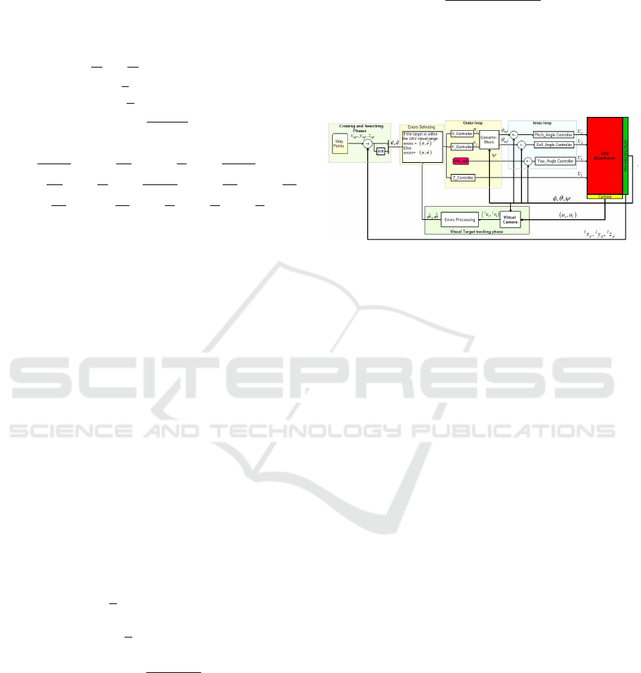
3.2 Controller Scheme
The full control scheme is proposed as a multi-loop,
Fig. 3. It is consisting of an inner loop that controls
attitude and an outer loop to control the yaw and the
translation.
The inner loop references are generated by the outer
loop using the following equations:
(
φ
re f
= arcsin (u
x
sin(ψ
d
) − u
y
cos(ψ
d
))
θ
re f
= arcsin
u
x
cos(ψ
d
)+u
y
sin(ψ
d
)
cos(φ
d
)
(11)
Regarding the outer loop, the position references are
obtained from the waypoints and the search trajectory
during the crossing and searching phases. While for
the tacking phase, the position and velocity errors are
obtained by vision (section 5).
Figure 3: Proposed Controller Scheme.
Concerning the control mode, an SMC based on
Exponential Reaching Law (ERL) is adopted due
to its robustness, low chattering effect and response
time.
3.3 Sliding Mode Controller Design
The considered system (10) is a second order, so the
sliding surface is given by:
S = ˙e + λe (12)
For attitude control, e ∈
e
φ
,e
θ
, ˙e ∈
˙e
φ
, ˙e
θ
,
e
φ
= e
1
= φ
d
− φ, e
θ
= e
3
= θ
d
− θ.
φ
d
/θ
d
are the desired QUAV’s attitude (46) and φ/θ
are the instantaneous QUAV’s attitude obtained by
IMU.
For the yaw control, e
ψ
= e
5
= ψ
d
− ψ, with ψ
d
is
the desired yaw, assumed to be constant and ψ the
instantaneous yaw obtained by IMU.
Concerning the horizontal and vertical position
control, the position errors (e
x
,e
y
,e
z
) and their deriva-
tives ( ˙e
x
, ˙e
y
, ˙e
z
) are not accessible since the QUAV’s
position/velocity references are those of the uncoop-
erative target.
Hence, the visual measurement detailed in (39), (44)
and (48) are used to define the relative sliding sur-
faces:
S
n
=
˙
ˆe
n
+ λ
n
ˆe
n
, n ∈
{
x,y, z
}
(13)
In order to design the controllers, an approximate
model called ”control model” (14) is used, rather than
defined in (10), in which the parameters uncertainty
ICINCO 2022 - 19th International Conference on Informatics in Control, Automation and Robotics
558

( ˜a
i
,
˜
b
i
), the measurements noise ( ˜x
i
) and the external
perturbations (d
•
) are considered.
˙
ˆx
1
= ˜x
2
˙
ˆx
2
= ˜a
1
˜x
4
˜x
6
+ ˜a
2
˜x
2
2
+
˜
b
1
U
2
+ d
φ
˙
ˆx
3
= ˜x
4
˙
ˆx
4
= ˜a
4
˜x
2
˜x
6
+ ˜a
5
˜x
2
4
+
˜
b
2
U
3
+ d
θ
˙
ˆx
5
= ˜x
6
˙
ˆx
6
= ˜a
7
˜x
2
˜x
4
+
˜
b
3
U
4
+ d
ψ
˙
ˆx
7
= ˜x
8
˙
ˆx
8
= ˜a
9
˜x
8
+
1
m
u
x
U
1
+ d
x
˙
ˆx
9
= ˜x
10
˙
ˆx
10
= ˜a
10
˜x
10
+
1
m
u
y
U
1
+ d
y
˙
ˆx
11
= ˜x
12
˙
ˆx
12
= ˜a
11
˜x
12
− g +
cos(φ)cos(θ)
m
U
1
+ d
z
(14)
With ˜x
i
= x
i
+ noise are the noisy measurement . d
•
,
• ∈
{
φ,θ, ψ,x,y,z
}
, with |d
•
| ≤ d
max
•
are the external
disturbances.
For simplification sake, the following expression
of (14) is adopted:
˙
˜x
i
= ˜x
i+1
˜
˙x
i+1
=
˜
f
i
(x) + ˜g
i
(x)U + d
•
e
i
= x
d
i
− x
i
(15)
i ∈
{
1,3, 5,7, 9,11
}
, U ∈
{
U
1
,U
2
,U
3
,U
4
,u
x
,u
y
}
, e
7
=
e
x
= x
d
− x, e
9
= e
y
= y
d
− y and e
11
= e
z
= z
d
− z
From (15), the first time derivative of the sliding sur-
face is given by:
˙
S = ¨x
d
i
−
˜
f ( ˜x) − ˜g( ˜x).U − d
•
+ λ. ˙e (16)
Using (16), the general form of the control law is
given by:
U =
1
˜g(x)
¨x
d
i
−
˜
f (x) + D
•
sign(S) + λ. ˙e −
˙
S
(17)
The term D
•
sign(S) is introduced to compensate the
external disturbance d
•
, such that:
d
max
•
< D
•
(18)
Defining the Lyapunov function :
V =
1
2
S
2
(19)
The first time derivative of V must be negative defined
to ensure the convergence,so:
˙
V = S
˙
S < 0 (20)
For ERL-based SMC,
˙
S is chosen as:
˙
S = −K
s
ign(S) − qS, q > 0,K > 0 (21)
Replacing (21) in (19), the control law is given by:
U =
1
˜g(x)
¨x
d
i
−
˜
f(x) + D
•
sign(S) + λ.˙e + Ksign(S ) + qS
(22)
This law forces the switching variable to reach the
switching surface at a constant rate K, but if K is
too small, the response time is important, on another
hand, a large K will cause a severe chattering. By
adding the proportional rate term Ksign(S), the state
is forced to approach switching manifold faster when
the sliding surface S is larger. (Liu, 2017).
For uncooperative target tracking, the desired ac-
celerations ¨x
d
, ¨y
d
, ¨z
d
are those of the target, which are
neither measurable nor estimable. Consequently, they
can be considered as a pounded perturbation, such
that:
| ¨x
d
(i)
| < ¨x
d
(i)max
= ∂
i
(23)
∂
i
> 0,i ∈
{
5,7, 9,11
}
Hence, the general expression of the outer loop
controller is given by:
U =
1
˜g(x)
−
˜
f (x) +
¯
D
•
sign(S) + λ. ˙e −
˙
S
(24)
In this case, the term
¯
D
•
sign(S) compensates the
external disturbance d
•
and the unknown acceleration
¨x
d
(i)
. Therefore, the constant
¯
D
•
must satisfy the fol-
lowing condition:
d
max
•
+ ∂
i
≤
¯
D
•
(25)
Thus, considering
˙
S as given in (24), the different con-
trol laws are summarized as follows:
U
2
=
1
˜
b
1
˙
S
θ
+ λ
θ
. ˙e
θ
+
¨
θ
d
− ˜a
4
˜x
2
˜x
6
− ˜a
5
˜x
2
4
+ D
θ
sign(S
θ
)
U
3
=
1
˜
b
2
˙
S
φ
+ λ
φ
. ˙e
φ
+
¨
θ
d
− ˜a
1
˜x
4
˜x
6
− ˜a
2
˜x
2
2
+ D
φ
sign(S
φ
)
U
4
=
1
˜
b
3
˙
S
ψ
+ λ
ψ
. ˙e
ψ
+
¨
ψ
d
− ˜a
7
˜x
2
˜x
4
− ˜a
8
˜x
2
6
+ D
ψ
sign(S
ψ
)
U
1
=
m
cos(φ)cos(θ)
˙
S
z
+ λ
z
.
ˆ
˙e
z
− ˜a
11
˜x
12
+ g +
¯
D
z
sign(S
z
)
u
y
=
m
U
1
˙
S
y
+ λ
y
.
ˆ
˙e
y
− ˜a
10
˜x
10
+
¯
D
y
sign(S
y
)
u
x
=
m
U
1
˙
S
x
+ λ
x
.
ˆ
˙e
x
− ˜a
9
˜x
8
+
¯
D
x
sign(S
x
)
(26)
Proof. Considering the expression of the control
model (14), then substituting (16) in the time deriva-
tion of the Lyapunov function, we get:
˙
V = S
¨x
d
i
−
˜
f ( ˜x) − ˜g( ˜x).U − d + λ. ˙e
(27)
For the quadcopter’s translation and yaw, replacing
the controller U by its expression given by (24) with
considering the
˙
S expression given in (21) , we get :
˙
V =
S
d + ¨x
d
i
− K|S| −
¯
D
•
|S| − qS
2
(28)
When: S < 0, (28) become :
˙
V = −
|S|
¨x
d
i
+ d
+ K|S| +
¯
D
•
|S| + qS
2
Under the condition (25), q > 0 and K > 0, it is clear
that:
˙
V < 0 (29)
Vision-based Sliding Mode Control with Exponential Reaching Law for Uncooperative Ground Target Searching and Tracking by
Quadcopter
559
When S ≥ 0, from (28) we get:
S
d + ¨x
d
i
−
¯
D
•
|S| ≤ −ε,ε ≥ 0
Hence:
˙
V <
−ε −
¯
D
•
|S| − qS
2
< 0 (30)
For the attitude control (φ and θ), the input control
U of (27) is replaced by the expression given in (17)
and following the same logic adopted for the transla-
tion’s stability proof, with taking in account condition
(18) instead of (25), the stability can be proved.
4 VISION MODELS DERIVATION
The vision modeling involves, the camera modeling
and the Camera Coverage Area (CCA) modeling.
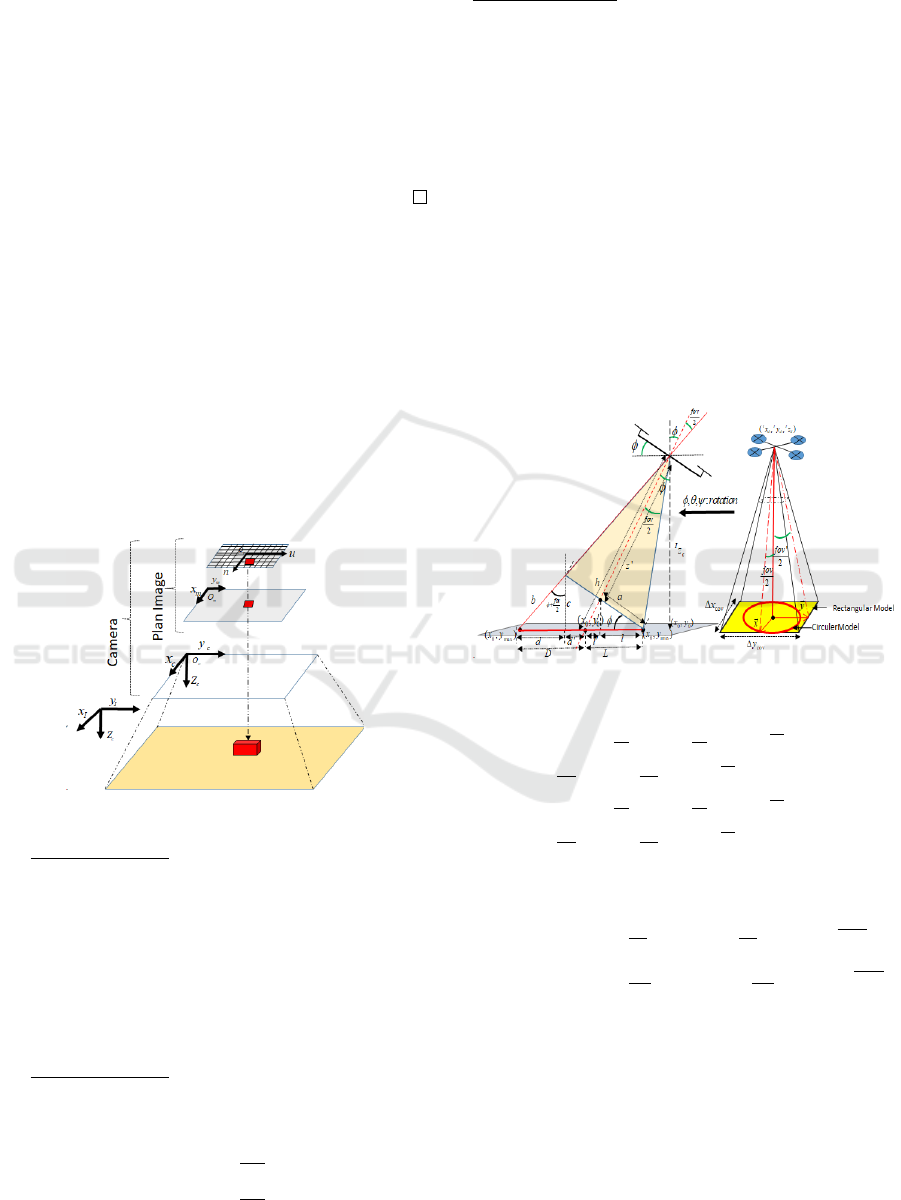
4.1 Camera Modeling
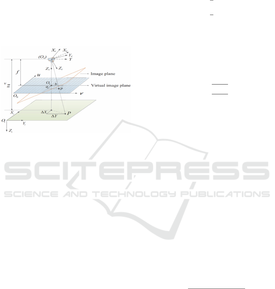
The pinhole model is adopted in this work due to
its simplicity and efficiency. It goes through three
elementary and successive transformations (Fig .4).
Figure 4: Projections for pinhole model.
Transformation 1: to express the coordinates
of the points characterizing the target
I
P
i
=
I
x
p
i
I
y
p
i
I
z
p
i
t
in the camera’s frame.
c
P
i
= R
C
I
P
i
−
I
O
c
. (31)
With
I
O
i
∈ ℜ
3
is the camera’s position in F
I
frame.
R
C
= R
t
is the rotation matrix between the F
I
and F
C
frames.
Transformation 2: is a perspective projection,
transforming point
c
P
i
into a two-dimensional point
in the image plane p
i
=
x
m
i
y
m
i
t
.
x
m
i
= f
c
x
p
i
c
z
p
i
y
m
i
= f
c
y
p
i
c
z
p
i
(32)
With f is the camera’s focal length.
Transformation 3: for the transformation from a met-
ric positioning to a pixel positioning
u
i
= k
x
x
m
i
+ u
0
n
i
= k
y
y
m
i
+ n
0
(33)
With (u
0
,n
0
) and k
x
/k
y
are the coordinates of the im-
age’s center and the number of pixels per unit of mea-
surement respectively.
4.2 Camera Coverage Area Modeling
The CCA is a calculated measure that defines theo-
retically the maximum visible region from a camera.
In the case of a rectangular modeling (Based on ge-
ometrical calculation) the CCA is limited by a rect-
angle centered in O
cca
I
x
cca
,
I
y
cca
and the maximal
distances covered along x and y axis are given by (35)
as depicted in Fig. 5 .
Figure 5: Camera Coverage Area Modeling.
I
x
cca
=
I
z
c
.T
f ov
2
S
θ
T
θ+
f ov
2
+C
θ
−
1
C
θ
C
ψ
−
I
z
c
.T
f ov
0
2
S
φ
T
φ+
f ov
0
2
+C
φ
−
1
C
φ
S
ψ
+
I
z
c
.T
θ
+
I
x
c
I
y
cca
=
I
z
c
.T
f ov
2
S
θ
T
θ+
f ov
2
+C
θ
−
1
C
θ
S
ψ
+
I
z
c
.T
f ov
0
2
S
φ
T
φ+
f ov
0
2
+C
φ
−
1
C
φ
C
ψ
+
I
z
c
.T
φ
+
I
y
c
(34)
∆x
cov
= 2.
I
z
c
.T
(
f ov
2
)
S
θ
c
T
(θ
c
+
f ov
2
)
+C
θ
c
+
1
2C
θ
c
∆y
cov
= 2.
I
z
c
.T
(
f ov
0
2
)
.
S
φ
c
T
(φ
c
+
f ov
0
2
)
+C
φ
c
+
1
2C
φ
c
(35)
T
= tan() and fov/fov’ are the height and the
width of the camera’s field of view.
For a circular modeling, the model is a circle centered
in C
0
with a rayon R
cca
, such that:
C
0
=
I
x
cca
,
I
y
cca
R
cca
= min(x
cov
,y
cov
)
(36)
For the detection model, the target is considered as
automatically detected once it entered into the CCA.
ICINCO 2022 - 19th International Conference on Informatics in Control, Automation and Robotics
560
5 TARGET POSITION AND
VELOCITY ESTIMATION
A virtual camera with its associated virtual frame
F
v
≡ (o
c
,~e
v
x
,~e
v
y
,~e
v
z
) are introduced, so that the origin
of the F
v
coincides with the origin of the real camera’s
frame, and its Z − axis ~e
v
z
is aligned with the optical
axis of the virtual camera, Fig 6.
Figure 6: Virtual camera concept.
The virtual camera inherits only the yaw, and the
horizontal translation of the real camera. By adopting
this technique, we can claim that any changes in the
image features are only due to the horizontal transla-
tion of the QUAV or to the target’s movement. There-
fore, the Horizontal Position’s Errors (HPE) and the
Velocity’s Errors (VE) between the QUAV and the
target are calculated using target image features ex-
pressed in the virtual camera. The same for the gen-
eration of the QUAV’s relative altitude.
5.1 Horizontal Position’s Errors
Estimation
Considering a set of points
c
P
i
∈ ℜ
3
characterizing
the target with their corresponding pixel coordinates
p
i
= (u
i
,n
i
). Then,
c
P
i
are projected in the virtual
image plane as follows (Jabbari et al., 2012):
v
u
i
v
n
i
= βR
t
φθ
u
i
n
i
f
(37)
β = f /
0 0 1
R
t
φθ
u
i
n
i
f
,R
t
φθ
=
R
θ
R
φ
t
Supposing that the target contains N > 3 non-
collinear feature points, the image’s feature centroid
v
p
g
= (
v
u
g
,
v
n
g
) in the virtual frame is given by:
v
u
g
=
1
N
N
∑
i=1
v
u
i
v
n
g
=
1
N
N
∑
i=1
v
n
i
(38)
The idea of the control scheme is to drive the QUAV
above the target, such that the desired virtual image’s
feature centroid is determined as the center of the vir-
tual image plane
v
p
g
=
v
p
0
.
Hence, from equations (38) and (37), the horizontal
position errors between the camera (QUAV) and the
target are given by:
(
ˆe
x
=
v
ˆz
v
u
g
−
v
u
0
f
ˆe
y
=
v
ˆz
v
n
g
−
v
n
0
f
(39)
Remark 1. ’
v
ˆz’ is the normal distance of the virtual
camera from the target, and is assumed to be equal to
the camera’s vertical position
I
ˆz
c
.
5.2 QUAV’s Altitude Reference
Generation
In a tracking scenario, the most intuitive and simple
approach is to fly the QUAV at a fixed altitude, which
must not be too high to ensure that the target is de-
tectable on the image plane, and must also not be too
low to ensure the visualization of all the target’s de-
tails. However, this approach cannot guarantee that
the QUAV flies at an optimal altitude. Thus, and
to ensure this optimality, the technique proposed by
(Zhang et al., 2020) to determine the desired QUAV’s
relative altitude is readopted in this work.
The proposed technique is summarized as follows:
- The introduction of a circle centered at O
c
with
radius r
opt
as an optimal observation zone in the
virtual image plane.
- Consider a circle centered at
v
p
g
and passing
through the farthest feature point of the target
(projected in the virtual plane) to cover the whole
target features. The circle radius r
trg
is given by:
r
trg
= max
(
r
(
v
u
i
−
v
u
g
)
2
+
(
v
n
i
−
v
n
g
)
2
)
,i = 1,., N
(40)
- Once the QUAV is above the target, its altitude
will be controlled through r
trg
which must be less
than or equal to the r
opt
to ensure that the target
stays within the optimal viewing area.
r
d
= υr
opt
,υ < 1. (41)
υ is the radius-scaling factor.
Vision-based Sliding Mode Control with Exponential Reaching Law for Uncooperative Ground Target Searching and Tracking by
Quadcopter
561

Considering the perspective projection, we get:
r
d
= f
d
trg
z
d
(42)
d
trg
is the unknown real distance between the
target center and the farthest target feature
point and z
d
is the desired QUAV’s altitude.
From (41) and (42) the desired vertical distance is
given by:
z
d
= r
trg
c
ˆz
p
υr
opt
(43)
Therefore, the vertical error is given by:
ˆe
z
=
c
ˆz
p
− z
d
(44)
In summary, the position errors are given by the fol-
lowing vector ∆ξ =
ˆe
x
ˆe
y
ˆe
z
t
.
5.3 Velocity Errors Estimation
To compute the velocity errors which is necessary for
the controller. The expression of the target’s feature
points
I
P
i
in the virtual frame is given by:
v
P
i
= R
ψ
I
P
i
−
I
O
v
(45)
Hence, the dynamic of the image features
v
˙p
i
=
v
˙u
i
v
˙n
i
t
corresponding to the set point
v
P
i
is ob-
tained by the first time derivation of equation (45)
considering that
v
z
p
i
=
c
z
p
i
=
c
z
p
.
v
˙u
i
v
˙n
i
=
1
v
z
p
i
f 0 −
v
u
i
0 f −
v
n
i
v
˙x
c
−
v
˙x
p
i
v
˙y
c
−
v
˙y
p
i
v
˙z
c
−
v
˙z
p
i
+
v
n
i
−
v
u
i
˙
ψ
(46)
The image feature dynamic given by (46) is rewritten
as follow:
v
˙p
i
=
c
ˆz
−1
p
A
i
v
∆v + B
i
˙
ψ (47)
Bearing in mind that the target feature points are
coplanar and have the same target linear velocity, it is
clear that in order to compute the three components of
the velocity errors
v
∆v, at least two points (i ≥ 2) are
needed. Finlay, the velocity errors expressed in the F
I
frame are given by:
∆v =
c
ˆz
p
R
t
ψ
A
+
(
v
˙p − B
˙
ψ) (48)
With ∆v =
ˆ
˙e
x
ˆ
˙e
y
ˆ
˙e
z
t
, A =
A
t
i
.. A
t
N
t
,
Q =
B
t
1
.. B
t
N
t
, A
+
is the Moore-
Penrose pseudo-inverse of matrix A and
v
˙p =
v
˙p
t
1
...
v
˙p
t
N
t
is obtained by measur-
ing the optic flow.
5.4 QUAV’s Relative Vertical Position
Measurement
Given the geometric models of the possible targets,
the horizontal distance between the camera and the
target is calculated using the image coordinates of
at least two target feature points and the correspond-
ing real distance between, obtained from the model
matching, them combined with equations (32) and
(33). It is given by:
c
ˆz
p
= f .D
i/ j
u
i
− u
j
k
x
2
+
n
i
− n
j
k
y
2
!
−1/2
(49)
D
i/ j
is the horizontal distance between two points
P
i
/P
j
on the target, obtained by model matching. u
i
/n
i
and u
j
/n
i
are their corresponding pixel coordinates.
6 SIMULATION AND
DISCUSSION
For the numerical simulations, the QUAV’s parame-
ters uncertainty is chosen such that ˜a
i
= a
i
± 15%a
i
and
˜
b
1
= b
i
± 15%b
i
.
The solver Runge-Kutta is used with a fixed-step
( 0.001 simpling rate).
Concerning the target, it is considered as a rect-
angular object, in which the visual features include
its four vertexes with the following coordinates (in
meters) (0.2,0.2, 0), (−0.2,0.2,0), (−0.2, −0.2,0)
and (0.2,−0.2, 0).
The camera position and attitude with respect to
F
B
frame are (0,0, 0.05)m and (0,0,0)rad respec-
tively.
The QUAV’s initial position and attitude are
(0,0, 0.1)m, (0,0,0)rad, respectively. The coor-
dinates of the starting point of the search phase is
(8,7, 0)m. The crossing and searching altitudes are
5m and 20m respectively. The searching trajectory is
a circle centered in the searching start point with a
rayon equal to R
CCa
.
The QUAV’s parameters uncertainty is chosen
such that ˜a
i
= a
i
± 15%a
i
and
˜
b
1
= b
i
± 15%b
i
. To
evaluate the visual measurement for the three flight
phases, we consider that the target is always visible
and the tracking process is started at the instant
t = 55s.
ICINCO 2022 - 19th International Conference on Informatics in Control, Automation and Robotics
562
0 20 40 60 80 100 120
t
0
50
100
Position error
e
x
e
y
e
z
0 20 40 60 80 100 120
t
-15
-10
-5
0
5
velocity error
de
x
de
y
de
z
Cross phase
Search phase
Track phase
Figure 7: Visual measurement: position and velocity errors
(with sign function).
0 20 40 60 80 100 120
t
0
50
100
Position errors
e
x
e
y
e
z
0 20 40 60 80 100 120
t
-10
-5
0
5
velocity errors
de
x
de
y
de
z
Cross phase
Search phase
Track phase
Figure 8: Visual measurement: position and velocity errors.
0 20 40 60 80 100 120
t
0
2
4
6
8
10
12
14
16
18
20
Z
p
Target/QUAV vertical distance
Z
p
-reel
Z
p
-estimated
Track phase
Search phase
Cross phase
Figure 9: Simulation results of the proposed Vision-based
vertical distance measurement (with sign function).
0 20 40 60 80 100 120
t
0
2
4
6
8
10
12
14
16
18
20
22
Z
p
Target/QUAV vertical distance
Z
p
-reel
Z
p
-estimated
Track phase
Search phase
Cross phase
Figure 10: Simulation results of the proposed Vision-based
vertical distance measurement.
0
0
5
10
15
Z
10
20
25
X
20
45
40
Y
35
30
30
25
20
15
40
10
5
0
Search phase
Track phase
Cross phase
Figure 11: Simulation results of the proposed flight scenario
in 3D.
0 5 10 15 20 25 30 35 40 45 50
X
0
5
10
15
20
25
30
35
40
45
50
Y
Cross phase
Search phase
Track phase
Figure 12: Simulation results of the proposed flight scenario
in 2D.
0 10 20 30 40 50 60 70 80 90 100
t
-1
0
1
Phi(rad)
Phi-ref
Phi
0 10 20 30 40 50 60 70 80 90 100
t
-1
0
1
Theta(rad)
Theta-Ref
Theta
0 10 20 30 40 50 60 70 80 90 100
t
-0.5
0
0.5
Psi(rad)
Psi-Ref
Psi
Track phase
Search phase
Cross phase
Figure 13: Simulation results of the QUAV’s attitude and
yaw control.
0 20 40 60 80 100 120 140 160
t
0
20
40
Xd
X-Ref
X-UAV
X-Traget
0 20 40 60 80 100 120 140 160
t
0
20
40
Yd
Y-Ref
Y-UAV
Y-Traget
0 20 40 60 80 100 120 140 160
t
0
10
20
Zd
Y-Ref
Y-UAV
Z-Traget
Track phase
Search phase
Cross phase
Figure 14: Simulation results of the QUAV’s translation
movement control.
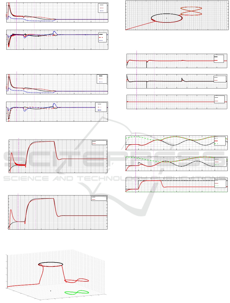
The simulation was performed by considering the
saturation function instead of the sign function in the
proposed controller, since the use of the saturation
function lead to a considerable improvement in the vi-
sual measurement results (Fig. 8 and Fig. 10), unlike
the sign function, which gave a noisy result, (Fig. 7
and Fig. 9).
The flight scenario is depicted in Fig. 11 and Fig. 12
(3D and 2D), in which the three flight phases are il-
lustrated: the cruise phase, the search phase and the
tracking phase. In Fig. 11 the automatic altitude tun-
ing is clearly depicted, where the QUAV has reduced
its altitude automatically for vision optimization.
For the control law results, Fig. 14 shows the control
results of the QUAV’s horizontal and vertical trajec-
tory. Figure. 13 exposes the QUAV’s attitude and yaw
control, where the chattering effect is too low.
Vision-based Sliding Mode Control with Exponential Reaching Law for Uncooperative Ground Target Searching and Tracking by
Quadcopter
563

7 CONCLUSION
The proposed strategy for uncooperative mobile
ground target tracking using a quadcopter has been as-
sessed using simulated scenarios. The evolved IBVS
approach allows improving searching, detection and
tracking efficiency while the proposed ERL based
Sliding mode controller guarantees the stability and
robustness of the QUAV. A simple searching law was
used for detecting a moving target and its relative
position and velocity estimation considering uncer-
tainties. Simulations were performed to successfully
demonstrate the performance and feasibility of the
proposed method.
REFERENCES
Borshchova, I. and O’Young, S. (2016). Visual servoing for
autonomous landing of a multi-rotor uas on a mov-
ing platform. Journal of Unmanned Vehicle Systems,
5(1):13–26.
Cantelli, L., Mangiameli, M., Melita, C. D., and Muscato,
G. (2013). Uav/ugv cooperation for surveying oper-
ations in humanitarian demining. In 2013 IEEE in-
ternational symposium on safety, security, and rescue
robotics (SSRR), pages 1–6. IEEE.
Cao, Z., Chen, X., Yu, Y., Yu, J., Liu, X., Zhou, C., and Tan,
M. (2017). Image dynamics-based visual servoing for
quadrotors tracking a target with a nonlinear trajectory
observer. IEEE Transactions on Systems, Man, and
Cybernetics: Systems, 50(1):376–384.
Chaumette, F. and Hutchinson, S. (2006). Visual servo con-
trol. i. basic approaches. IEEE Robotics & Automation
Magazine, 13(4):82–90.
Ding, X. C., Rahmani, A. R., and Egerstedt, M. (2010).
Multi-uav convoy protection: An optimal approach to
path planning and coordination. IEEE transactions on
Robotics, 26(2):256–268.
Duggal, V., Sukhwani, M., Bipin, K., Reddy, G. S., and Kr-
ishna, K. M. (2016). Plantation monitoring and yield
estimation using autonomous quadcopter for precision
agriculture. In 2016 IEEE international conference on
robotics and automation (ICRA), pages 5121–5127.
IEEE.
Fink, G., Xie, H., Lynch, A. F., and Jagersand, M. (2015).
Experimental validation of dynamic visual servoing
for a quadrotor using a virtual camera. In 2015 In-
ternational conference on unmanned aircraft systems
(ICUAS), pages 1231–1240. IEEE.
Jabbari, H., Oriolo, G., and Bolandi, H. (2012). Dynamic
ibvs control of an underactuated uav. In 2012 IEEE In-
ternational Conference on Robotics and Biomimetics
(ROBIO), pages 1158–1163. IEEE.
Janabi-Sharifi, F. and Marey, M. (2010). A kalman-filter-
based method for pose estimation in visual servoing.
IEEE transactions on Robotics, 26(5):939–947.
Liu, J. (2017). Sliding mode control using MATLAB. Aca-
demic Press.
Menouar, H., Guvenc, I., Akkaya, K., Uluagac, A. S.,
Kadri, A., and Tuncer, A. (2017). Uav-enabled intelli-
gent transportation systems for the smart city: Appli-
cations and challenges. IEEE Communications Mag-
azine, 55(3):22–28.
Pestana, J., Sanchez-Lopez, J. L., Saripalli, S., and Campoy,
P. (2014). Computer vision based general object fol-
lowing for gps-denied multirotor unmanned vehicles.
In 2014 American Control Conference, pages 1886–
1891. IEEE.
Prabhakaran, A. and Sharma, R. (2021). Autonomous in-
telligent uav system for criminal pursuit–a proof of
concept. The Indian Police Journal, page 1.
Puri, A. (2005). A survey of unmanned aerial vehicles (uav)
for traffic surveillance. Department of computer sci-
ence and engineering, University of South Florida,
pages 1–29.
Radiansyah, S., Kusrini, M., and Prasetyo, L. (2017). Quad-
copter applications for wildlife monitoring; iop con-
ference series: Earth and environmental science.
Samad, T., Bay, J. S., and Godbole, D. (2007). Network-
centric systems for military operations in urban ter-
rain: The role of uavs. Proceedings of the IEEE,
95(1):92–107.
Wang, Z., Gao, Q., Xu, J., and Li, D. (2022). A review
of uav power line inspection. Advances in Guidance,
Navigation and Control, pages 3147–3159.
Zhang, K., Shi, Y., and Sheng, H. (2021). Robust nonlin-
ear model predictive control based visual servoing of
quadrotor uavs. IEEE/ASME Transactions on Mecha-
tronics, 26(2):700–708.
Zhang, S., Zhao, X., and Zhou, B. (2020). Robust vision-
based control of a rotorcraft uav for uncooperative tar-
get tracking. Sensors, 20(12):3474.
ICINCO 2022 - 19th International Conference on Informatics in Control, Automation and Robotics
564
