
Linear Programming: A Diet Problem with Methane Emission
Xunzi Xie
1,*
, Shi Zhang
2
, Yizhe Chen
3
and Yifan Pan
4
1
University of California, Los Angeles, 90024, U.S.A.
2
Shanghai Pinghe School, Shanghai, 201206, China
3
Hangzhou Foreign Language School, Hangzhou, 310000, China
4
Villanova Preparatory School, Ojai, 93023, U.S.A.
Keywords: Linear Programming, Optimization, Diet Problem, Methane Emissions.
Abstract: Cattle diet problems are concerned with finding the optimal diet for cattle. Classical diet problems are linear
programming problems. This paper considers a complication of diet problem, adding to the traditional setting
the extra component of methane emission. We find that under proper assumptions this complicated model is
yet another linear programming problem. We then realize our model with empirical data and obtain the
optimal diet for cattle via the simplex method. Sensitivity analysis is run against selected parameters. We
conclude that our model is mostly successful, yielding many practical considerations.
1 INTRODUCTION
Diet, by its definition, is the food and drink that a
person or animal drinks and eats regularly.
Researches have been done on optimizing the diet of
cattle in a limited range or within a specific area. To
generalize, we developed an adaptable model which
aims at balancing between the cost of a diet and
maintaining the animal’s basic conditions. The
general goal of this process is getting the maximum
nutritional requirements for the least amount of
money. A unique feature of our model is the added
goal of reducing methane emissions.
In building the model, we have made
assumptions, gathered data for nutrition intake
required for cattle, formulated functions, and gained
results by utilizing linear programming.
2 BACKGROUND AND
PROBLEM SET-UP
First we present a quick summary of our problem
scenario. Our model starts with a cattle representative
which is bought in at an initial weight. This cattle
gains weight daily. The cattle is fed with a diet of N
types of food. That cattle is also assumed to have a
realistic eating habit, where it eats only a certain
amount of food every day determined by its weight.
This value is known as the dry matter intake of the
cattle.
For each type of food, a set of nutrient
concentrations are obtained from laboratory and
empirical estimations. 4 nutrient requirements are
checked every day to ensure that the cattle is growing
healthily. The daily growth in weight of the cattle
depends on how much food the cattle consumes, and
in particular we assume that the growth in weight
depends on the total energy intake of the cattle.
Ultimately the main source of income of the cattle
owner comes from selling the finishing cattle. The
sale price is per unit weight.
Finally, IPCC estimated the daily methane
emission of cattle as a linear function of its total
energy intake (Dong, Mangino, & McAllister 2006).
We then imagine that the government imposes
environmental policies so that an emission fine is
charged for every unit of excessive methane emission
(amount that exceeds an emission threshold).
We move on to formulate the above scenario into
an optimization problem. First, recall that our
objectives are to increase the sale price of cattle, to
reduce methane emission, and to reduce the diet cost.
We then translate these into the following equation:
𝑚𝑎𝑥. 𝑝 ∙ ∆𝑊 − 𝑐
∙𝑥−𝑓∙𝑀
(1)
where ∆𝑊 is the daily increase of weight, 𝑐
(Rankin, 2021, Halopka, 2020, Livestock, Poultry, &
Grain, University of Missouri Extension,
IndexMundi, Alibaba 2021) is a vector of diet food
Xie, X., Zhang, S., Chen, Y. and Pan, Y.
Linear Programming: A Diet Problem with Methane Emission.
DOI: 10.5220/0011361000003438
In Proceedings of the 1st International Conference on Health Big Data and Intelligent Healthcare (ICHIH 2022), pages 295-301
ISBN: 978-989-758-596-8
Copyright
c
2022 by SCITEPRESS – Science and Technology Publications, Lda. All rights reserved
295
cost, 𝑓 is the unit fine charged on methane emission
𝑀
, 𝑝 (Ag Decision Maker 2021) is the unit sell price
of cattle, and 𝑥 is a vector of the weight of each food
type in the diet. The given question requires us to vary
𝑥 to achieve the maximum of the objective function
of 𝑥 defined above.
To ensure that this problem is realistic, we set up
six constraints with respect to the food vector 𝑥 .
First, obviously entries of 𝑥 should be positive:
𝑥≥0 (2)
We introduce the term 𝐷 to represent the daily
dry matter intake of a cattle, which is estimated using
the linear equation 𝐷 = 1.8545 + 0.01937 ∙ 𝑊
where 𝑊
is the initial weight (Ag Decision Maker
(2021). 𝐷 then equals the total weight of the food
provided:
𝑒
∙ 𝑥 = 𝐷, 𝑒 =
1, 1, … ,1
(3)
We require that our diet should satisfy the daily
nutrient requirements of cattle. We introduce the
matrix 𝐴 (National Academy of Science,
Engineering, and Medicine (2000), whose columns
correspond to each food type and rows correspond to
the different types of nutrients. We further introduce
the term 𝑏 National Academy of Science,
Engineering, and Medicine (2000) to represent the
minimum nutrients required by the cattle for
sustenance. Hence,
𝐴∙𝑥≥𝑏 (4)
We also require that the cattle are always gaining
weight. This ensures that the farmer is always making
profit. According to NASEM, the daily increase in
weight can be estimated as ∆𝑊 = 13.91 ∙
(
𝐸
−
𝐸
)
∙𝑊
.
, where 𝑊 is the daily weight, 𝐸
is
the total energy intake, and 𝐸
is the energy required
to maintain a cattle’s activities. 𝐸
and 𝐸
can
further be estimated by 𝐸
=𝐶
∙𝑥 and 𝐸
=𝑠∙
𝑊
.
, where 𝐶 National Academy of Science,
Engineering, and Medicine (2000) is an energy vector
specifying the energy concentration in each type of
food and 𝑠 National Academy of Science,
Engineering, and Medicine (2000) is a scaling factor
depending on the cattle’s breed, sex, and cattle’s
nutritional conditions etc. These equations then allow
us to write ∆𝑊 as a function of 𝑥 , and we obtain
another constraint:
∆𝑊
(
𝑥
)
= 13.91 ∙
(
𝐶
∙𝑥 −𝑠∙𝑊
.
)
∙𝑊
.
≥0(5)
According to IPCC, the total methane emission
𝑀 is estimated as 𝑀=
∙∙
, w h e r e 𝑘 is a unit
conversion factor, 𝑚 is a methane conversion factor,
and 𝑚𝑒𝑐 is the methane energy constant (Dong,
Mangino, & McAllister, 2006). We then set an
emission threshold 𝑀
and define the corresponding
excessive methane emission 𝑀
=𝑀−𝑀
. Our
problem is meaningful only if 𝑀
is positive:
𝑀
≥0 (6)
We also want to ensure that 𝑀
follows IPCC’s
empirical estimation:
𝑀
≥
∙∙
−𝑀
=
∙
∙𝐶
∙𝑥−𝑀
(7)
Combining these estimates, we obtain the
following optimization problem:
(*) 𝑚𝑎𝑥. 𝑝 ∙ ∆𝑊(𝑥) − 𝑐
∙𝑥−𝑓∙𝑀
(8)
𝑠. 𝑡. 𝑥 ≥ 0, 𝑒
∙𝑥=𝐷,𝐴∙𝑥≥𝑏,∆𝑊
(
𝑥
)
≥0,𝑀
≥0,𝑀
≥
∙
∙𝐶
∙𝑥−𝑀
(9)
A summary of all variables and their symbols can
be found in table 1.
Table 1: Symbols
Symbol Uni
t
Description
𝑥
kg N-dimensional vector specifying how much kg of each food types a cattle eats per day.
𝑀
kg Estimated kg of methane emitted by a cattle per day
𝑐
$/kg N-dimensional vector specifying how much a kg of each food type costs
𝐴
unit MN matrix specifying how much nutrient each food type contains
𝑏
kg M-dimensional vector specifying daily requirement of a specific nutrient
𝐶
J/kg N-dimensional vector specifying energy concentration in each food type
𝑒
unit N-dimensional vector of ones
ICHIH 2022 - International Conference on Health Big Data and Intelligent Healthcare
296
𝑝
$/kg Selling price of cattle meat
𝑊
kg Daily weight of a cattle
𝑓
$/kg Amount of capital punishment per kg of excessive methane emission
𝐷
kg Daily dry matter intake of a cattle
𝐸
MCal Daily energy of maintenance for a cattle
𝑠
J/kg0.75 Correlation factor between Emand W, which depends on breed, nutritional state, and sex etc.
𝑘
MJ/MCal Unit conversion factor
𝐸
MCal Total energy intake of a cattle per day
𝑚
unit Methane conversion factor
𝑚𝑒𝑐
MJ/kg Methane energy constant
𝑀
kg Methane emission threshold
3 DATA AND METHODOLOGY
3.1 Data
Our primary data sources are IPCC and NASEM.
Other data (mainly market prices of diet food and
cattle) are quoted from various Internet sources. We
manually assign values to some parameters, such as
the fine placed on excessive methane emissions. See
table 2-4 for a full presentation of data and their
sources.
Table 2: Nutritional/Energy concentration and Cost (A/C
and c):
Food Type
NE
(Mcal/kg)
CP
(%)
C
(%)
P
(%)
Cost
($/ton)
ALFALFA
Fresh
1.38 18.90 1.29 0.26 167
Hay 1.31 18.6 1.40` 0.28 171
Straw 0.6 4.40 0.30 0.07 70
Gluten
meal
2.20 66.3 0.07 0.61 700
Seed 2.24 24.4 0.17 0.62 370
Barley
Grain
2.06 13.2 0.05 0.35 114
Sugar beets 1.76 9.8 0.68 0.1 125
Cotton
hulls
0.68 4.2 0.15 0.09 230
Wheat
midds
1.6 18.7 0.17 1.01 220
Cottonseed
Meal
1.79 46.1 0.02 0.02 370
Distiller’s
grains
dried
2.18 30.4 0.26 0.83 271
Oat hulls 0.41 4.1 0.16 0.15 129
Table 3: Nutritional requirement (b): (assume W_0 = 400
kg; breed code “1 Angus”; W_T = 890 kg).
Type Measurement/Unit (per day) Value
Energy Net Energy (NE) / Mcal 6.38
Table 4: Data Sources.
Protein
Metabolizable protein
(MP) /kg
(CP = MP/0.64)
0.274
C/Calciu
m
C / kg 9/1000
P/Phosphorus P / kg 7/1000
Paramete
r
Estimated Value/Unit Source
Linear Programming: A Diet Problem with Methane Emission
297
𝑐
See table 2
𝐴
See table 2 NASEM
2000, 134
𝑏
See table 3 NASEM
2000, 106
𝐶
See table 2 NASEM
2000, 134
𝑝
2.9548/$/kg
𝑊
400/kg NASEM
2000, 106
𝑓
88644/1000000 30% of
sell
p
rice
𝑠
0.077 NASEM
2000, 6
𝑘
4184000/1000000
/
𝑚
3% IPCC
2006,
4 ,10.30
𝑚𝑒𝑐
55.65 IPCC
2006, 4,
10.31
𝑀
0.125 Assume
𝐸
=𝐸
then
compute
IPCC’s
e
q
uation
3.2 Methodology
Simplex Method is an iterative algorithm, which aims
to find the optimal solution of x. Its main steps are:
1) find a basic feasible solution;
2) judge whether the solution is the optimal
according to the optimality theory;
3) if it is the optimal, then stop the process;
4) if it is not, then try to generate a new feasible
solution which better minimizes the objective
function; and
5) judge its optimality again.
This loop is continued until an optimal solution is
found.
However, in different cases, there are distinct
results of the simplex method. In some cases, the LP
problem would degenerate. This happens when one
of basic feasible variables has zero value. Infinite
iterations would appear, and this prevents the
algorithm from converging.
If no degeneracy appears, the simplex method
would converge after certain iterations. Two results
would appear: an optimal feasible solution, which
leads to a minimum value of objective; or an infinite
amount of feasible solutions where the objective has
no lower bound.
Simplex method only works for optimization
problems in their canonical forms. To convert (*) into
its canonical form, we define the canonical variables
as follows:
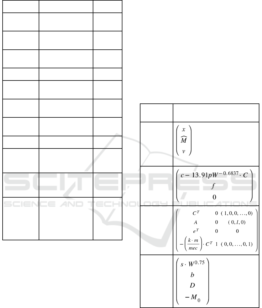
Table 5: Canonical Variables.
Slack
Variable
Definition
x
(where v is a vector of slack
variables
)
c
A
b
These canonical variables define an optimization
problem as follows:
(**) 𝑚𝑖𝑛. 𝑐̂
∙𝑥
𝑠. 𝑡. 𝑥≥0,𝐴
∙𝑥=𝑏
(10)
And it is easy to check that (**) is equivalent with
(*). We then run the simplex method to obtain a
ICHIH 2022 - International Conference on Health Big Data and Intelligent Healthcare
298
solution to (**), from which we obtain a solution to
(*).
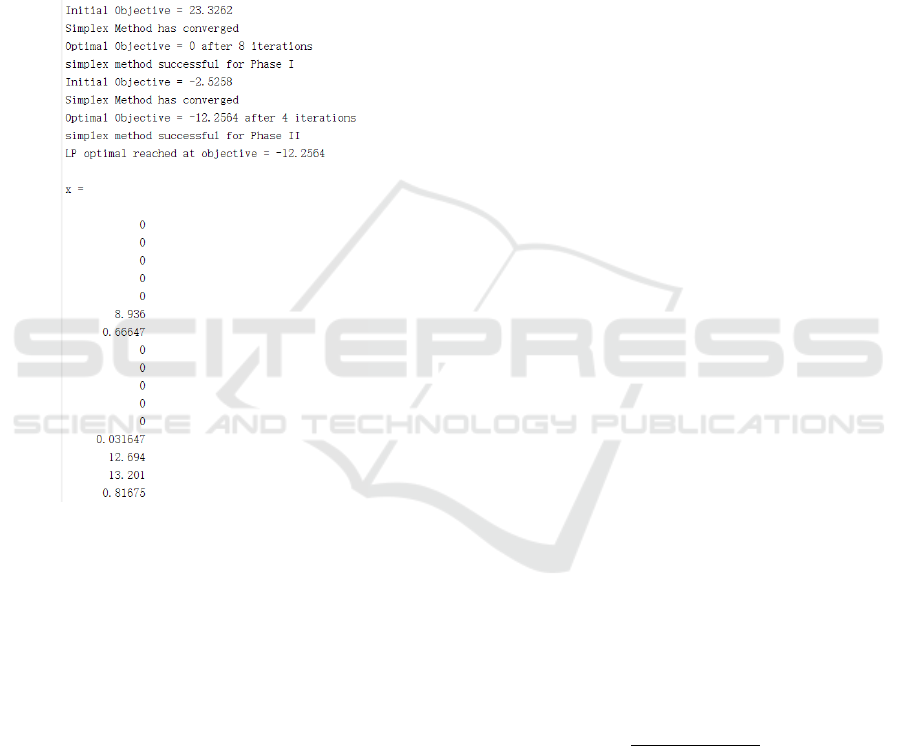
3.3 Results and Analysis
The algorithm run on the data apparently converges
and outputs an optimal diet with two non-zero
components: about 8.9 kg of barley grains and 0.67
kg of sugar beets. The program also reports an
optimal objective of -12.2564, meaning that the
maximum profit for the cattle owner on the first day
is about 12 dollars.
Figure 1: Simplex Method Status and Optimal 𝒙
.
A couple of remarks on the result are in place.
First, only two types of food are included in the
optimal diet. Usually one should worry when the
number of non-zero outputs is small. In particular, it
may mean that the problem is degenerate if the
number of non-zero outputs is significantly lower
than the number of constraints. However, for our
problem we only have one equality constraint in our
original diet problem:
𝑒
∙ 𝑥 = 𝐷 (11)
Hence if the other inequality constraints are
merciful, then potentially we only need to allow one
or a few degrees of freedom in the diet vector x to
meet all the constraints. This intuition is justified.
Observe that 𝑥 has five other non-zero components.
One of these corresponds to 𝑀
, and the other four are
slack variables. Indeed, 𝐴
in the canonical form is a
rank 7 matrix. Hence, it makes sense for us to obtain
exactly seven non-trivial components in our solution.
The fact that only two components of the diet vector
are non-trivial is a direct consequence of the way the
constraints are formulated. Therefore,
mathematically the result is consistent.
There are two zero slack variables. This indicates
that two constraints have reached the boundaries on
the feasibility plane. When we plug in our vector x
back to the optimization problem, we can see that the
requirement of Calcium (C) is exactly reached. If the
cattle may require slightly more protein, phosphorus,
and energy, the diet given above is still suitable and
effective. But if calcium (C) requirement increases,
then the boundary is pushed outwards and the
optimum diet above no longer satisfies the nutrient
requirements.
Another legitimate concern is that compared with
the nutrient requirements specified in vector 𝑏, some
reasonably priced food types are simply too nutritious
so that the nutrient requirements are easily met. This
intuition can be backed up by a simple sensitivity
analysis on the parameter 𝑏 . Indeed, apparently
doubling 𝑏 only increases the maximum profit by
about 0.1 dollars. The new optimal diet is still
composed of sugar beets and barley grains where
barley grains. This pattern persists as we impose
stricter nutrient requirements, until when the nutrient
requirements are about four times stricter than the
original one and the linear program then becomes
infeasible. Therefore, the objective function is
apparently insensitive to the nutrient requirements
(wherever the problem is feasible). This then supports
the intuition that when the cattle owner is choosing
between different types of diet food with the hope of
maximizing net profit, nutrient requirements turn out
to be a rather insignificant factor.
Next, observe that the thirteenth component (of
which corresponds to 𝑀
) is closed to 0. This means
that the optimal methane emission is very closed to
the emission threshold (𝑀
). Recall that methane
emission and growth in weight both depend linearly
on energy intake:
(***) 𝑓=
.∙∙
.
∙
∙
(12)
So, changing 𝑥 should result in comparable
changes in the profit generated by growth in weight
𝑝∙𝑊 and the cost resulted from excessive methane
emission −𝑓 ∙ 𝑀
. Sensitivity analysis on 𝑝 a n d 𝑓
confirms a part of this intuition. The objective is
sensitive to 𝑝 but quite stable with respect to 𝑓 ,
unless f is multiplied to be quite large. This makes
sense intuitively, since 𝑓 is per kg charge on
Linear Programming: A Diet Problem with Methane Emission
299

methane emission. As we all know methane is a gas,
and hence kg is a rather misleading dimension of
weight for methane.
Furthermore, when the profit generated by growth
in weight matches with the cost from emission (the
exact 𝑓 that makes this happen can be obtained from
solving the equation (***) above) the farmer is not
making any real profit out of the cattle business. This
is perhaps a useful fact for governors to decide how
much fine should be in place (with respect to the sale
price of cattle) in order to economically effectively
affect the cattle owner’s behaviors.
Finally, sensitivity analysis on the food cost 𝑐
and 𝐷 are also conducted. The food cost is
apparently very low in comparison with sale price 𝑝
and methane emission fine. Hence, apparently the
objective is quite insensitive to the food cost unless
the sale price of cattle diet food becomes comparable
to the sale price of cattle itself. 𝐷 acts as an upper
bound for the diet vector 𝑥 . Should D increase
drastically, it is expected that under our problem set
up the cattle grows in weight indefinitely. The
objective indeed shoots off as D increases
indefinitely.
4 RESULTS AND ANALYSIS
In this paper, we have considered a revised cattle diet
problem with the added component of methane
emissions. We formulate the problem as an
optimization problem and solve it through the
simplex method. In general, our problem is easy to
construct and solve. Sensitivity analysis proves that
the methane emission fee is an effective way to affect
the cattle business. In addition, our model is also
adaptable to different species of animals and different
nutrition requirements, by simply changing several
parameters in our model. Within reasonable range,
we expect our method to still converge to an optimal.
Any model has to give way to simplifications. We
now turn to point out some issues and suggestions for
future improvements. To begin with, there are a
couple of assumptions that can be avoided by
considering more complicated models. First, in our
model we assume that the weight gain of the cattle is
a constant. Our model can naturally be extended to a
dynamic programming problem by introducing a
weight function that evolves over discrete time.
Moreover, we assume that the same nutrient
requirements apply to cattle among all age groups. In
reality, it requires more nutrients when cattle are
young and in the process of growth. Hence the
constraint for nutrient requirements should depend on
time as well, and this can be incorporated with the
growth in weight in a dynamic programming version
of our simply model.
Also, note that the methane emission fee we put
on is regarded as fixed regardless of the amount of
excessive emissions. However, as in the case of
taxation capital punishments are typically piecewise
functions. This can be potentially a more complex
constraint for our problem.
Finally, in our optimal diet only two types of food
are selected. This is because our constraints and
nutritional estimations are simple and we pay no
attention to digestion processes and finer nutritional
requirements. For example, our system is based on an
assumption that the cattle will take in all the nutrition
the food supplies them. However, in the real world it
is definitely not the truth. The cattle may require other
food to help them fully absorb the nutrients. Future
studies of cattle diet problems should take these into
the account and consider, for example, a more
intricate mechanistic model of cattle’s nutrition.
5 CONCLUSIONS
Our group formulates a revised diet problem, which
considers sell price of cattle, cost of the diet, the fine
charged on methane emission, and the weight growth
of cattle. We obtain formulas mainly from NASEM
and IPCC and collect data of parameters on the
Internet. This could then be solved by Simplex
Method in Matlab. We conclude with a suggested
optimal diet and suggest for future research that a
dynamic version of our problem to be developed.
REFERENCES
Ag Decision Maker (2021). Historical Cattle Prices.
https://www.extension.iastate.edu/agdm/livestock/pdf/
b2-12.pdf
Alibaba.com (2021). Organic Price Sugar Pellets Beet Pulp.
https://ua1335743999cerh.trustpass.alibaba.com/produ
ct/62006362618-
810718723/Organic_Price_Sugar_Pellets_Beet_Pulp.h
tml
AMS Livestock, Poultry, & Grain Market News. US
(2021). Hay Auction Weighted Average Report For
June 23,
2021.https://www.ams.usda.gov/mnreports/ams_1725.
pdf
Dong, H., Mangino, J., & McAllister, T. (2006). Emissions
from Livestock and Manure Management. In: IPCC
(Ed.), 2006 Guidelines for National Greenhouse Gas
Inventories. The Institutes for Global Environmental
ICHIH 2022 - International Conference on Health Big Data and Intelligent Healthcare
300

Strategies, Japan. volume 4.10: pp. 31-
32.https://www.ipcc-
nggip.iges.or.jp/public/2006gl/pdf/4_Volume4/V4_00
_Cover.pdf
Halopka, R. US (2020). Hay Market Demand and Price
Report for the Upper Midwest For January 13,
2020.https://fyi.extension.wisc.edu/forage/files/2020/0
1/01-13-20.pdf
IndexMundi (2021). Barley Monthly Price.
https://www.indexmundi.com/commodities/?commodi
ty=barley&months=60
National Academy of Science, Engineering, and Medicine
(2000). Nutrient Requirements of Beef Cattle: Seventh
Edition. National Academy Press. p.6, pp.106-134.
Rankin, M. US (2021). USDA Hay Market.
https://hayandforage.com/articles.sec-7-1-
Markets.html
University of Missouri Extension. US (2021). By-Product
Feed Price Listing.
http://agebb.missouri.edu/dairy/byprod/bplist.asp
Linear Programming: A Diet Problem with Methane Emission
301
