
Reward Prediction for Representation Learning
and Reward Shaping
Hlynur Davíð Hlynsson and Laurenz Wiskott
Institut für Neuroinformatik, Ruhr-Universität Bochum, Universitätsstraße 150, Bochum, Germany
Keywords:
Reinforcement Learning, Representation Learning, Deep Learning, Machine Learning.
Abstract:
One of the fundamental challenges in reinforcement learning (RL) is the one of data efficiency: modern
algorithms require a very large number of training samples, especially compared to humans, for solving en-
vironments with high-dimensional observations. The severity of this problem is increased when the reward
signal is sparse. In this work, we propose learning a state representation in a self-supervised manner for re-
ward prediction. The reward predictor learns to estimate either a raw or a smoothed version of the true reward
signal in an environment with a single terminating goal state. We augment the training of out-of-the-box RL
agents in single-goal environments with visual inputs by shaping the reward using our reward predictor during
policy learning. Using our representation for preprocessing high-dimensional observations, as well as using
the predictor for reward shaping, is shown to facilitate faster learning of Actor Critic using Kronecker-factored
Trust Region and Proximal Policy Optimization.
1 INTRODUCTION
Deep learning has enjoyed great success in recent
years with a fortunate combination of larger data sets,
increasing computational capabilities and advances in
algorithm design in addition to an ample offering of
flexible software ecosystems. In particular, reinforce-
ment learning (RL), which is the discipline of ma-
chine learning concerned with general goal-directed
behavior. RL has shown great promise since Deep-
Mind combined the principles of RL with deep learn-
ing to achieve human-like skill on Atari video games
(Mnih et al., 2013). Since then, the list of games
where machine triumphs over man grows longer with
the addition of algorithms surpassing human capabil-
ities in games such as Go, (Silver et al., 2016), Poker
(Brown and Sandholm, 2019) and a restricted version
of DOTA 2 (Berner et al., 2019).
Even though the dominance of humans is being
tested by RL agents on numerous fronts, there are
still great difficulties for the field to overcome. For in-
stance, the data that is required for algorithms to reach
human performance is on a far larger scale than that
needed by humans. Furthermore, the general intelli-
gence of humans remains unchallenged. Even though
an RL agent has reached superhuman performance in
one field, its performance is usually poor when it is
tested in new areas.
The study of methods to overcome the problem of
data efficiency (Hlynsson et al., 2019) and transfer-
ability of RL agents in environments where the agent
must reach a single goal is the focal point of this work.
We consider a simple way of learning a state represen-
tation by predicting either a raw or a smoothed ver-
sion of a sparse reward yielded by an environment.
The two objectives, learning a representation and pre-
dicting the reward, are directly connected as we train
a deep neural network for the prediction and the hid-
den layers of this network learn a reward-predictive
representation of the input data.
The reward signal is created by collecting data
from a relatively low number of initial episodes using
a controller that acts randomly. The representation is
then extracted from an intermediate layer of the pre-
diction model and re-used as general preprocessing
for RL agents, to reduce the dimensionality of visual
inputs. The agent processes inputs corresponding to
its current state as well as the desired end state, which
is analogous to mentally visualizing a goal before at-
tempting to reach it. This general approach of relying
on state representations, that are learned to predict the
reward rather than maximizing it, has been motivated
in the literature (Lehnert et al., 2020) and we show
that our representation is well-suited for single-goal
environments. Our work adds to the growing body
of knowledge related to deep unsupervised (Hlynsson
Hlynsson, H. and Wiskott, L.
Reward Prediction for Representation Learning and Reward Shaping.
DOI: 10.5220/0010640200003063
In Proceedings of the 13th International Joint Conference on Computational Intelligence (IJCCI 2021), pages 267-276
ISBN: 978-989-758-534-0; ISSN: 2184-3236
Copyright © 2023 by SCITEPRESS – Science and Technology Publications, Lda. Under CC license (CC BY-NC-ND 4.0)
267

and Wiskott, 2019) and self-supervised (Schüler et al.,
2018) representation learning .
We also investigate the effectiveness of augment-
ing the reward for RL agents, when the reward is
sparse, with a novel problem-agnostic reward shap-
ing technique. The reward predictor, which is used
to train our representation, is not only used as a part
of an auxiliary loss function to learn a representation,
but it is also used during training the RL system to
encourage the agent to move closer to a goal loca-
tion. Similar to advantage functions in the RL litera-
ture, given the trained reward predictor, the agent re-
ceives an additional reward signal if it moves from
states with a low predicted reward to states with a
higher predicted reward. We find this reward augmen-
tation to be beneficial for our test environment with
the largest state-space.
2 BACKGROUND
2.1 Markov Decision Processes
A partially-observable Markov decision process
(POMDP) is a tuple
(S ,A,P ,R ,P(s
0
),Ω,O,γ) (1)
which we also refer to as the environment.
The environment starts in a state s ∈ S drawn from
P(s
0
), from which the agent interacts sequentially
with the environment by choosing action a
t
from ac-
tion space A at time steps t.
Given the agent’s state s
t
and action a
t
, the transi-
tion function P governs the next state s
t+1
. The agent
receives an observation o
t
∈ Ω, determined by the ob-
servation function O, and a reward r
t
, determined by
the reward function R .
A discount factor γ ∈ (0,1) is usually included in
the definition of POMDPs and it comes into play in
the optimization function of the agent. Namely, the
objective of an RL agent is to learn a policy π that
determines the behavior of the agent in the environ-
ment by mapping states to a probability distribution
over A, written π(a, s) = P(a
t
= a|s
t
= s). The policy
should maximize the expected discounted future sum
of rewards, or the expected return:
R
Σ
=
∞
∑
t=0
γ
t
r
t
(2)
2.2 Reward Shaping
Sparse rewards in environments is a common problem
for RL agents. The agent’s goal is to associate its in-
puts with actions that lead to high rewards, which can
be a lengthy process if the agent only rarely experi-
ences positive or negative rewards.
Reward shaping (Mataric, 1994) is a popular
method of modifying the reward function of an MDP
to speed up learning. It is useful for environments
with sparse rewards to augment the training of the
agent but skillful applications of reward shaping can
in principle aid the optimization for any environ-
ment – although the efficacy of the reward shaping
is highly dependent on the details of the implemen-
tation (Amodei and Clark, 2016). In the last few
years, reward shaping has been shown to be use-
ful for complex video game environments, such as
real-time strategy games (Efthymiadis and Kudenko,
2013) and platformers (Brys et al., 2014) and it has
also been combined with deep neural networks to im-
prove agents in first person shooter games (Lample
and Chaplot, 2017).
As an illustration, consider learning a policy for
car racing. If the goal is to train an agent to drive op-
timally, then supplying it with a positive reward for
reaching the finish line first is in theory sufficient.
However, if it is punished for actions that are never
beneficial, for instance crashing into walls, it priori-
tizes learning to avoid such situtations, allowing it to
explore more promising parts of the state space.
Furthermore, just reaching the goal is insufficient
if there is competition. To make sure that we have a
winning racer, a small negative reward can be intro-
duced at every time step to urge the agent to reach the
finish line quickly. Note that the details of the reward
shaping in this example requires domain knowledge
from a designer who is familiar with the environment.
It would be more generally useful if the reward shap-
ing would be autonomously learned, just as the policy
of the agent, as we propose to do in this work.
2.3 Reward-predictive/Maximizing
Representations
(Lehnert et al., 2020) make the distinction be-
tween reward-maximizing representations are reward-
predictive representations. They argue how reward-
maximizing representations can transfer poorly to
new environments while reward-predictive represen-
tations generalize successfully. Take the simple grid
world navigation environments in Figure 1, for exam-
ple. The agent starts at a random tile in the grid and
gets a reward of +1 by reaching the rightmost column
in Environment A or by reaching the middle column
in Environment B. The state space in Environment A
can be compressed from the 3 × 3 grid to a vector of
length 3, [φ
p
1
,φ
p
2
,φ
p
3
] of reward-predictive representa-
NCTA 2021 - 13th International Conference on Neural Computation Theory and Applications
268

tions. To predict the discounted reward, it suffices to
describe the agent’s state with φ
p
j
if it is in the jth row.
0 0 1
0 0 1
0 0 1
0 1 0
0 1 0
0 1 0
Environment A
Environment B
Available
actions:
State Representation
Optimal action
Figure 1: Reward-maximizing vs. reward-predictive
representations. In this grid world example, the agent
starts the episode at a random location and can move up,
down, left, or right. The episode ends with a reward of 1
and terminates when the agent reaches the rightmost col-
umn. Both the reward-predictive representation and reward-
maximizing representation φ
p
and φ
m
, respectively, are use-
ful for learning the optimal policy in Environment A. The
reward-predictive representation φ
p
collapses each column
into a single state to predict the discounted future reward.
The reward-maximizing representation φ
m
makes no such
distinction as moving right is the optimal action in any state.
It is a different story if the representations are transfered to
Environment B, where reaching the middle column is now
the goal. The representation φ
p
can be reused and the op-
timal policy is found if agent now takes a step left in φ
p
3
.
However, the representation φ
m
is unable to discriminate
between the different states and is useless for determining
the optimal policy.
The reward-maximizing representation for Envi-
ronment A is much simpler: the whole state space can
be collapsed to a single element φ
m
, with the optimal
policy of always moving to the right. If these rep-
resentations are kept, then the reward-predictive rep-
resentation φ
p
is informative enough for a RL agent
to learn how to solve Enviroment B. The reward-
maximizing representation φ
m
has discarded too many
details of the environment to be useful for solving this
new environment.
2.4 Successor Features
The successor representation algorithm learns two
functions: the expected reward R
SF
π
received after
transitioning into a state s, as well as the matrix
M
SF
π
of discounted expected future occupancy of each
state, assuming that the agent starts in a given state
and follows a particular policy π. Knowing the quan-
tities R
SF
π
and M
SF
π
allows us to rewrite the value func-
tion:
V
π
(s) = E
s
0
R
SF
π
(s)M
SF
π
(s,s
0
)
(3)
The motivation for this algorithm is that it com-
bines the speed of model-free methods, by enabling
fast computations of the value function, with the flex-
ibility of model-based methods for environments with
changing reward contingencies.
This method is made for small, discrete envi-
ronments but it has been generalized for continuous
environments with so-called feature-based successor
representations, or successor features (SFs) (Barreto
et al., 2016). The SF algorithm similarly calcu-
lates the discounted expected representation of future
states, given the agent takes the action a in the state s
and follows a policy π:
ψ
π
(s,a) = E
π
"
∞
∑
t=0
γ
t−1
φ
t+1
|s
t
= s,a
t
= a
#
(4)
where φ is some state representation. Both the SF ψ
and the representation φ can be deep neural networks.
3 RELATED WORK
3.1 Reward-predictive Representations
(Lehnert et al., 2020) compare successor features
(SFs) to a nonparametric Bayesian predictor that
is trained to learn transition and reward tables for
the environment, either with a reward-maximizing
or a reward-predictive loss function. (Lehnert and
Littman, 2020) prove under what conditions suc-
cessor features (SFs) are either reward-predictive or
reward-maximizing (see distinction in Section 2.3).
They also show that SFs work succesfully for transfer
learning between environments with changing reward
functions and unchanged transition functions, but
they generalize poorly between environments where
the transition function changes.
Our work is distinct from the reward-predictive
methods that they compare as our representation does
not need to calculate expected future state occupancy,
as is the case for SFs. Our method scales better
for more complicated state-spaces because we do not
tabulate the states, as they do with their Bayesian
model, but learn arbitrary continuous features of high-
dimensional input data. In addition to that, learning
our reward predictor is not only a "surrogate" objec-
tive function as we use it for reward shaping as well.
3.2 Reward Shaping
The advantages of reward shaping are well under-
stood in the literature (Mataric, 1994). A recent trend
in RL research is the study of methods that can learn
the reward shaping function in an automatic manner,
without the need of (often faulty) human intervention.
Reward Prediction for Representation Learning and Reward Shaping
269
(Marashi et al., 2012) assume that the environment
can be expressed as a graph and that this graph formu-
lation is known. Under these strong assumptions, they
perform graph analysis to extract a reward shaping
function. More recently, (Zou et al., 2019) propose
a meta-learning algorithm for potential-based auto-
matic reward shaping. Our approach is different from
previous work as we assume no knowledge about the
environment and train a predictor to approximate (po-
tentially smoothed) rewards, which is then used to
construct a potential-based reward shaping function.
3.3 Goal-conditioned RL
(Kaelbling, 1993) studied environments with multiple
goals and small state-spaces. In their problem setting,
the agent must reach a known but dynamically chang-
ing goal in the fewest number of moves. The observa-
tion space is of a low enough dimension for dynamic
programming to be satisfactory in their case. (Schaul
et al., 2015) introduce the Universal Value Function
Approximators and tackle environments of larger di-
mensions by learning a value function neural network
approximator that accepts both the current state and
a goal state as the inputs. In a similar vein, (Pathak
et al., 2018) learn a policy that is given a current state
and a goal state and outputs an action that bridges the
gap between them. (Hlynsson et al., 2020) learn a
predictable representation that is paired with a repre-
sentation predictor and combine it with graph search
to find a given goal location. In contrast to these ap-
proaches, we learn a reward-predictive representation
in a self-supervised manner which is used to prepro-
cess raw inputs for RL policies.
4 APPROACH
In this section, we explain our approach mathemati-
cally. Intuitively, we train a deep neural network to
predict either a raw or a smoothed reward signal from
a single-goal environment. The output of an inter-
mediate layer in the network is then extracted as the
representation – for example, by simply removing the
top layers of the network. The full reward predictor
network is used for reward shaping by rewarding the
agent for moving from lower predicted values toward
higher predicted values of the network.
4.1 Learning the Representation
Suppose that f
θ
: R
c
→ [0, 1] is a differentiable func-
tion parameterized by θ and c is a positive integer.
We use f
θ
to approximate the discounted return in a
POMDP with a sparse reward: the agent receives a
reward of 0 for each time step except when it reaches
a goal location, at which point it receives a positive
reward and the episode terminates.
Given an experience buffer D =
{(s
t
,a
t
,r
t
,s
t+1
)
i
}, we create a new data set
D
∗
= {(s
t
,a
t
,r
∗
t
,s
t+1
)
i
}. The new rewards are
calculated according to the equation
r
∗
t
= γ
m
r
t+m
(5)
where γ ∈ [0,1] is a discount factor and M > m > 0
is the difference between t and the time step index
of the final transition in that episode, for some max-
imum time horizon M. Throughout our experiments,
we keep the value of the discount factor equal to 0.99
and we train on D or D
∗
.
Assume that our differentiable representation
function φ : R
d
→ R
c
is parameterized by θ
0
and maps
the d-dimensional raw observation of the POMDP to
the c-dimensional feature vector. We train the rep-
resentation for the discounted-reward prediction by
minimizing the loss function
L( f
θ
[φ
θ
0
(s
t+1
)],r
∗
t
) = (r
∗
t
− f
θ
[φ
θ
0
(s
t+1
)])
2
(6)
with respect to the parameters θ of f and the parame-
ters θ
0
of φ over the whole data set D
∗
. See Figure 2
for a conceptual overview of our representation learn-
ing.
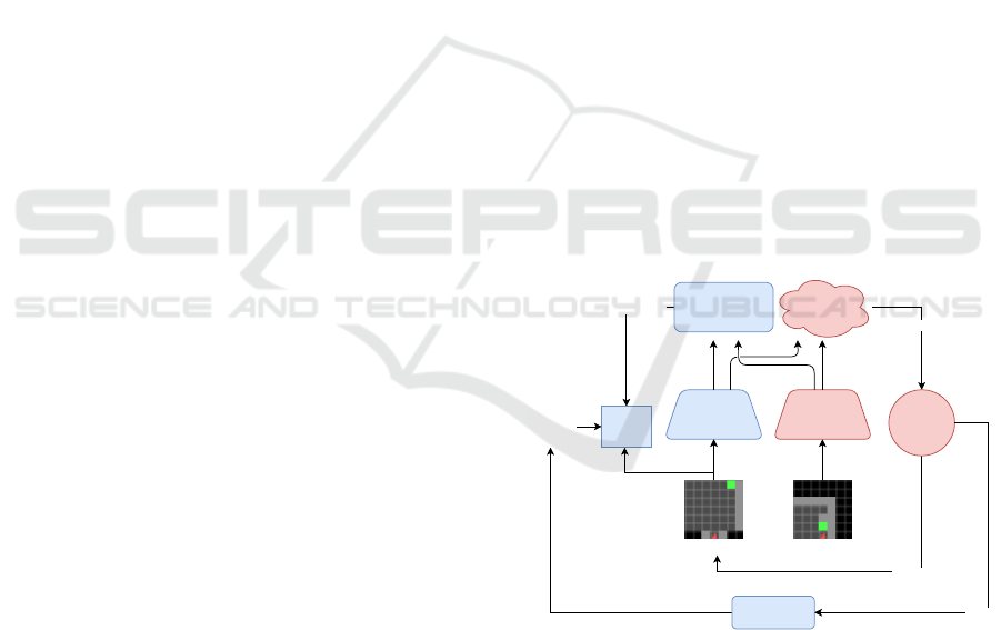
Representation Representation
Action
Policy
Prediction
Reward Predictor
Loss
fuction
Current state Goal state
Smoothed
Reward
New state
Environment
Reward
smoothing
Reward
Figure 2: Learning and Using the Representation. Our
representation and reward predictor is trained with the ele-
ments highlighted in blue. The trained representation is then
used for dimensionality reduction for an RL agent, that in-
teracts with the environment as indicated by the elements
highlighted in red.
4.2 Reward Shaping
(Ng et al., 1999) define a reward shaping function F
as potential-based if there exists a function f : S → R
such that for all states s,s
0
∈ S the equation holds:
NCTA 2021 - 13th International Conference on Neural Computation Theory and Applications
270

F(s, a, s
0
) = γ f (s
0
) − f (s) (7)
and γ is the MDP’s discount factor. They prove
for single-goal environments that every optimal pol-
icy for the MDP M = (S ,A, P ,R ,P(s
0
),γ) is also
optimal for its reward-shaped counterpart M
0
=
(S ,A, P ,R + F,P(s
0
),γ), and vice versa. They also
show, for a given state space S and action space A,
that if F is not potential-based, then there exist a tran-
sition function P and a reward function R such that
no optimal policy in M
0
is optimal in M.
We would like our reward shaping function to
be potential-based (Equation 7) to reap the theoreti-
cal advantages and propose a potential-based reward
shaping function based on the reward predictor
F(s, a, s
0
) =
γ f
θ
(φ
θ
0
[s
0
]) − f
θ
(φ
θ
0
[s])
(H − I)/H
= γ f
∗
(s
0
) − f
∗
(s)
(8)
where f
∗
= f
θ
(φ
θ
0
[s
0
])(H −I)/H, f
θ
is the reward pre-
dictor and φ
θ
0
is our representation from the previous
section. Note that both f
θ
and φ
θ
0
are assumed to be
fully trained before the policy of the agent is trained,
for example using data gathered by a random policy,
but they can in principle also be updated as the policy
is being learned. The factor (H − I)/H scales down
the intensity of the reward shaping where I ∈ N
+
is
the number of episodes that the agent has experienced
and H ∈ N
+
is the maximum number of episodes
where the agent is trained using reward shaping. The
strength of the reward shaping is the highest in the be-
ginning to counteract potentially adverse effects of er-
rors in the reward predictor. It is also more important
to incentivize moving toward the general direction of
the goal in the early stages of learning, after which the
un-augmented reward signal of the environment is al-
lowed to "speak for itself" and guide the learning of
the agent toward the goal precisely.
5 METHODOLOGY AND
IMPLEMENTATION
5.1 Environment
The method is tested on 3 different gridworld envi-
ronments based on the Minimalistic Gridworld Envi-
ronment (MiniGrid) (Chevalier-Boisvert et al., 2018).
Tiles can be empty, occupied by a wall or occupied
by lava. The constituent states of S are determined by
the agent’s location and direction (facing north, west,
south or east), along with the goal’s location. The
steps taken since the episode’s initialization is also
(a) Full World States.
(b) Agent’s Point of View.
(c) Goal Observations.
Figure 3: Two-Room Environment. The red agent must
reach the green goal in as few steps as possible. The agent
starts each episode between the two rooms, facing a random
direction (up, down, left or right). Each column corresponds
to a snapshot of 1 episode. The light tiles correspond to
what the agent sees while the dark tiles are unseen by the
agent. (a) Examples of the full state (b) The observation
from the agent’s current state (c) A goal observation. This
is the agent’s point of view from a state that separates the
agent from the goal by 1 action.
tracked for reward calculations. See Figure 3a for 3
different world states in one of our environments.
The action space A has 3 actions: (1) turn left,
(2) turn right and (3) move forward. The transition
function is deterministic. The agent relocates to the
tile it faces if it moves forward and the tile is empty
and nothing happens if the tile is occupied by a wall.
The episode terminates if the tile is occupied by lava
or the goal. The agent rotates in place if it turns left or
right. Reaching the green tile goal gives a reward of
1 − 0.9 ·
#steps taken
#max steps
, other actions give no reward. The
environment times out after #max step = 100 steps.
The discount factor is γ = 0.99.
We consider the following three environments:
5.1.1 Two-room Environment
The world is a 8 × 17 grid of tiles, split into two
rooms, where walls are placed at different locations
to facilitiate discrimination between the rooms from
the agent’s point of view. (Figure 3). The agent is
placed between the two rooms, facing a random di-
rection. The goal is at 1 of 3 possible locations. This
Reward Prediction for Representation Learning and Reward Shaping
271

is a modified version of the classical four-room envi-
ronment layout (Sutton et al., 1999).
5.1.2 Lava Gap Environment
In this environment, the agent is in a 4 × 4 room with
a column of lava either 1 or 2 spaces in front of the
agent (Figure 4) with a gap in a random row. The
agent always starts in the upper left corner and the
goal is always in the lower right corner.
Figure 4: The Lava Gap Environment. The red agent
must reach the green goal in as few steps as possible while
avoiding the orange lava tiles.
5.1.3 Four-room Environment
An expansion to the two-room environment with two
additional rooms (Figure 5) and both the agent and
the goal location are placed at random locations.
Figure 5: Four-Room Environment. The agent and goal
locations are randomized in each episode. The 7 × 7 grid of
highlighted tiles in front of the agent is the observation.
5.2 Baselines
We combine our representations with two RL al-
gorithms as implemented in Stable Baselines (Hill
et al., 2018) using the default hyperparameters: (1)
Actor Critic using Kronecker-Factored Trust Region
(ACKTR) (Wu et al., 2017) and a version of the Prox-
imal Policy Optimization (PPO2) algorithm (Schul-
man et al., 2017).
For both algorithms, 6 variations are compared:
(1) ACKTR / PPO2 with raw image inputs (Deep
RL), (2) inputs are preprocessed with successor fea-
tures (SF), (3) inputs are preprocessed using our rep-
resentation, trained on raw reward predictions (Ours
1r), (4) the input is preprocessed using our represen-
tation and the reward is shaped, trained on raw re-
ward predictions (Ours 1r + Shaping), (5) the input
is preprocessed using our representation, trained on
smoothed reward predictions (Ours 64r), (6) the in-
put is preprocessed using our representation and the
reward is shaped, trained on smoothed reward predic-
tions (Ours 64r + Shaping). Care has been taken to
ensure that each model has the same architecture and
number of parameters.
5.3 Model Architectures
Every model is realized as a neural network using
Keras (Chollet et al., 2015). Below, the representa-
tion and policy networks are used for our method and
the SF comparison, the reward prediction network is
used only for our method and the deep RL network is
used only for the deep RL comparison, where the RL
algorithm also learns the representation.
The Representation Networks: are two convolu-
tional networks with a 28 × 28 × 3 input. The first
layer discards every other column and row. This is
followed by 8 filters of size 3 × 3 with a stride of 3.
This is followed with a ReLU activation and a 2 × 2
max pooling layer with a stride of 2. The pooling
layer’s output is passed to a layer with 16 convolu-
tional filters of size 3×3 and a stride of 2 and a ReLU
activation. The output is passed to a linear dense layer
with 16 units, defining the dimension of the represen-
tation. No zero padding is applied in any layer.
The Policy Networks: are 3-layer fully-connected
networks accepting the concatenated output of the
representation network for the agent’s current point of
view and the goal observation as input. The first two
layers have 64 units and a ReLU activation and the
last layer has 3 units and a linear activation function.
The three units represent the three actions left, right,
and forward in a one hot encoding. Winner takes all
is used to decide on the action.
Our Reward Prediction Network: is a 3-layer fully-
connected network with the same input as the pol-
icy network: the concatenated representation of the
agent’s current view and the goal observation. The
first two layers have 256 units and a ReLU activation
but the last layer has 1 unit and a logistic activation.
The Deep RL Network: stacks the representation
network and the policy network on top of each other.
The representation network accepts the input and out-
puts the low-dimensional representation to the policy
network that outputs the action scores.
5.4 Training the Representation and
Predictor Networks
We collect a data set of 10 thousand transitions by
following a random policy in the two-room environ-
ment. For this data collection, each episode has a 50%
NCTA 2021 - 13th International Conference on Neural Computation Theory and Applications
272
chance to have the goal location in the bottom room
or on the left side of the top room (see the left and
middle pictures in Figure 3a). The reward predictor
and the representation are trained in this manner for
all experiments, including the lava gap and the four-
room environment. Thus, we use a representation and
reward predictor that have never seen lava. For the ex-
periments with smoothed rewards, the sparse reward
associated with the observations in the data set is aug-
mented by associating a new reward to the 64 states
leading to observations with a positive reward using
Equation 5 with a discount factor of 0.99. Ater the re-
ward has been (potentially) smoothed in this way, ob-
servations associated with a positive reward are over-
sampled 10 times to balance the data set, regardless
of whether the reward has been augmented or not.
6 RESULTS AND DISCUSSION
6.1 Two-room Environment
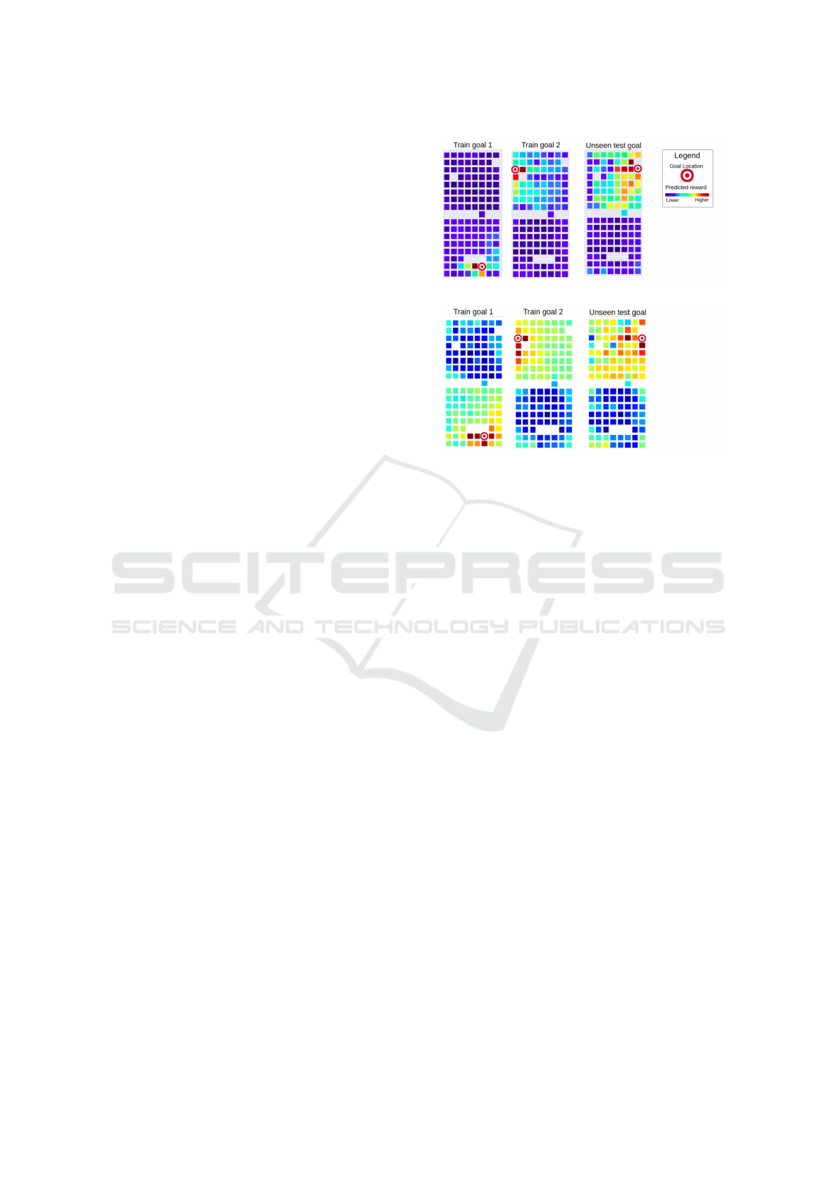
We start by visualizing the outputs of our reward pre-
dictor in the rooms, depending on the goal location, in
Figure 6. Each square indicates the average predicted
reward for transitioning to the corresponding tile.
The predicted reward spikes in a narrow region
around the two goal locations that were used to train
the raw reward predictor (Figure 6a), but the area of
states with high predicted rewards is wider around
the test goal. This difference is due to overfitting on
the specific training paths that were more frequently
taken toward the respective goals, but this does not
harm the generalization capabilities of the network.
The peakyness of the predictions disappears when the
predictor is trained on the smoothed rewards (Figure
6b). However, higher predicted rewards in the cor-
ner of the other room appear. Both scenarios, raw
and smoothed reward prediction, show promise for
the application of reward shaping under our training
scheme, as the agent benefits from finding neighbor-
hoods with higher values of predicted reward until it
reaches the goal, instead of relying on a sparse reward
that is only given when the agent lands on the goal.
In Figure 7, we illustrate the variance of the mean
reward (left side) and the variance of the optimal per-
formance (right side) of the different methods, as a
function of the time steps taken for training. We aver-
age over 10 runs and in each run we perform 10 test
rollouts, so each point is the aggregate of 100 episodes
in total. The error bands indicate two standard devia-
tions. This methodology of generating the plots also
applies to Figure 9, Figure 10 and Figure 11.
(a) Raw reward prediction.
(b) Smoothed reward prediction.
Figure 6: Predicted Rewards, Two-room environment.
The predictor is trained on the setups shown on the left and
in the middle, and tested for the setup on the right.
The learning curves of ACKTR and PPO2 get
close to a mean reward of 1 the fastest using our rep-
resentations. There no significant benefit from us-
ing smoothed reward shaping for ACKTR, and the
raw reward shaping is in fact harmful in this case.
For PPO2, the agent using our representation that is
trained on raw reward predictions learns the fastest.
Regular deep RL is clearly outperformed by the vari-
ants that use reward-predictive representations. We
believe that this is because RL agents can generally
benefit from the input being preprocessed, as the com-
putational overhead for learning the policy is reduced.
This effect is enhanced when the preprocessing is
good, which is the case for our representation: it ab-
stracts away unnecessary information as it trained to
output features that indicate the distance between the
agent and the goal, when the goal is in view.
The difference in the performance of a method on
the left hand side vs. the right hand side can be ex-
plained due to systematically different behaviors. For
example, an agent might be poor at searching for the
goal, giving it low average mean rewards, but it takes
the direct course to the goal when it sees it, giving it
a good average minimum episode length.
Reward Prediction for Representation Learning and Reward Shaping
273
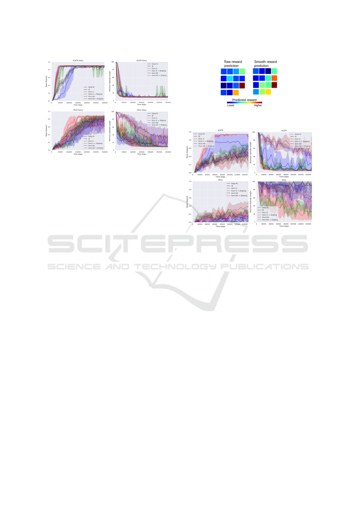
Figure 7: Two-room Environment. In these experiments,
there are only two rooms and the agent must reach a goal
that is always at the same location.
6.2 Lava Gap Environment
6.2.1 Learning from Scratch
The heatmaps of average predicted rewards are visu-
alized in Figure 8. The reward predictor was trained
on the two-room environment. The tiles closest to
the goal have the highest values, with a particularly
smooth gradient toward the goal for the smoothed-
reward predictor, which demonstrates that there is
potential gain from transfering the prediction-based
reward shaping between similar environments. The
learning performance of the different methods can be
seen in Figure 9. The decidedly fastest learning can
be observed when the actor-critic method is combined
with our representation, trained on raw reward predic-
tions and without reward shaping. Regular deep RL is
the second-best but with a very large variance on the
performance. Our reward shaping variations and the
SFs are very close in performance, albeit significantly
worse than the other two. The poor performance of
reward shaping can be explained by the fact that there
are very few states, which makes the reward shap-
ing unnecessary in such a simple environment. All
the methods look more similar when PPO2 optimiza-
tion is applied, with respect to the mean rewards, but
our variant that is trained on smooth reward prediction
and uses reward shaping reaches the highest average
performance in the last iterations.
6.2.2 Transfer Learning
To investigate how the methods compare for adapting
to new environments, we trained the policies for 8000
steps on the two-room environment before learning
to solve the lava gap environment, see Figure 10. Our
Figure 8: Predicted Rewards, Lava Gap. Average pre-
dicted reward per state in the lava gap environment.
Figure 9: Lava Gap Experiment. All policies learn to
solve the lava gap environment from scratch.
method, without reward shaping, facilitates the fastest
learning for ACKTR in this case. Deep RL is the most
severely affected by this change, which is probably
due to the method learning a reward-maximizing rep-
resentation in one environment that does not transfer
well to another environment. Every PPO2 variation
looks bad for this scenario, but smooth-reward predic-
tion representation with reward shaping has the high-
est mean reward and our raw-reward prediction rep-
resentation has the lowest average minimum episode
length.
6.3 Four-room Environment
In our final comparison, we add two additional rooms
to the two-room environment and randomize both the
goal location and the starting position of the agent,
with the results shown in Figure 11. Looking at the
minimum episode lengths, for the ACKTR learner,
our raw-reward prediction representation with reward
shaping performs best and the one without reward
shaping comes in second. There is little discernible
difference between the performance of SFs and Deep
RL, but they both perform significantly worse than
our methods. The scale of the mean reward is a great
deal lower than in the previous experiments since the
NCTA 2021 - 13th International Conference on Neural Computation Theory and Applications
274
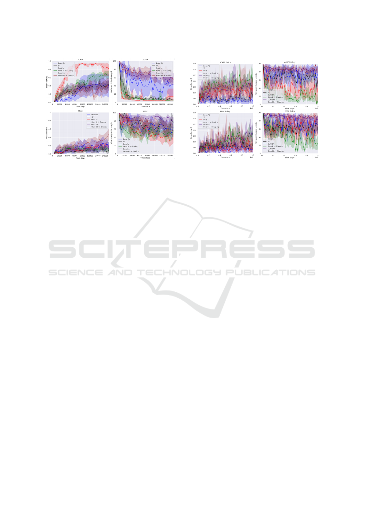
Figure 10: Re-learning Experiment The policies are
trained for 8 thousand training steps on the two-room envi-
ronment before being trained on the lava gap environment.
average distance between the starting tile of the agent
and the goal is much larger than in the previous two
environments.
For this scenario, all the methods look similarly
bad for the PPO2 policy, except for our raw-reward
representations, with reward shaping, which has the
lowest minimum episode length. The big advantage
of reward shaping in this environment compared to
the two-room environment can be explained by the in-
creased complexity, making the reward shaping more
helpful in guiding the agent’s search. In the previ-
ous experiments, the agent and goal locations start at
fixed locations, allowing the agents to solve it by rote
memorization. The reward shaping function calcu-
lated by the raw-reward predictor fares significantly
better in this situation. We hypothesize that this is
due to the smoothed-reward predictor distracting the
agent by pushing it to corners, as the visualization in
Figure 6b would suggest.
The reward shaping given by the raw-reward pre-
dictor is more discriminative, as we see in Figure 6a.
The agent receives a positive reward as soon as the
goal reaches its point of view, which is any location
up to 6 tiles in front of it and no further than 3 tiles
away from it to the left or to the right. This allows the
reward shaping function to guide the agent directly to
the goal, assuming that they are in the same room and
that there is no wall obstructing the agent’s field of
vision.
7 CONCLUSION
Processing high-dimensional inputs for reinforcement
learning agents remains a difficult problem, especially
if the agent must rely on a sparse reward signal to
Figure 11: Full Four-room Environment. The agent and
goal are placed at random locations at the start of each
episode.
guide its representation learning. In this work, we put
forward a method to help alleviate this problem with a
method of learning representations that preprocesses
visual input for reinforcement learning (RL) methods.
Our contributions are (i) a reward-predictive repre-
sentation that is trained simultaneously with a reward
predictor and (ii) a reward shaping technique using
this trained predictor. The predictor learns to approx-
imate either the raw reward signal or a smoothed ver-
sion of it and it is used for reward shaping by encour-
aging the agent to transition to states with higher pre-
dicted rewards.
We used a view of the goal as a second input for
the methods in our experiments, but this is in princi-
ple not necessary as moving toward the green tile as it
becomes visible is sufficient. Removing the goal in-
put might encourage the agents to learn policies that
scan all the rooms faster until the goal reaches its field
of vision.
We have shown the usefulness of our represen-
tation and our reward shaping scheme in a series of
gridworld experiments, where the agent receives a vi-
sual observation of its goal as input along with an
observation of its immediate surroundings. Prepro-
cessing the input using this representation speeds up
the training of two out-of-the-box RL methods, Ac-
tor Critic using Kronecker-Factored Trust Region and
Proximal Policy Optimization, compared to having
these methods learn the representations from scratch.
In our most complicated experiment, combining our
representation with our reward shaping technique is
shown to perform significantly better than the vanilla
RL methods, which hints at its potential for success,
especially in more complex RL scenarios.
Reward Prediction for Representation Learning and Reward Shaping
275

ACKNOWLEDGEMENT
We would like to thank Moritz Lange for his valuable
contribution to the preparation of this paper.
REFERENCES
Amodei, D. and Clark, J. (2016). Faulty reward
functions in the wild. https://blog.openai.com/
faulty-reward-functions/,2016.
Barreto, A., Dabney, W., Munos, R., Hunt, J. J., Schaul,
T., Van Hasselt, H., and Silver, D. (2016). Successor
features for transfer in reinforcement learning. arXiv
preprint arXiv:1606.05312.
Berner, C., Brockman, G., Chan, B., Cheung, V., D˛ebiak,
P., Dennison, C., Farhi, D., Fischer, Q., Hashme,
S., Hesse, C., et al. (2019). Dota 2 with large
scale deep reinforcement learning. arXiv preprint
arXiv:1912.06680.
Brown, N. and Sandholm, T. (2019). Superhuman ai for
multiplayer poker. Science, 365(6456):885–890.
Brys, T., Harutyunyan, A., Vrancx, P., Taylor, M. E.,
Kudenko, D., and Nowé, A. (2014). Multi-
objectivization of reinforcement learning problems by
reward shaping. In 2014 international joint confer-
ence on neural networks (IJCNN), pages 2315–2322.
IEEE.
Chevalier-Boisvert, M., Willems, L., and Pal, S. (2018).
Minimalistic gridworld environment for openai gym.
https://github.com/maximecb/gym-minigrid.
Chollet, F. et al. (2015). Keras. https://keras.io.
Efthymiadis, K. and Kudenko, D. (2013). Using plan-based
reward shaping to learn strategies in starcraft: Brood-
war. In 2013 IEEE Conference on Computational In-
teligence in Games (CIG), pages 1–8. IEEE.
Hill, A., Raffin, A., Ernestus, M., Gleave, A., Kanervisto,
A., Traore, R., Dhariwal, P., Hesse, C., Klimov, O.,
Nichol, A., Plappert, M., Radford, A., Schulman, J.,
Sidor, S., and Wu, Y. (2018). Stable baselines. https:
//github.com/hill-a/stable-baselines.
Hlynsson, H. D., Schüler, M., Schiewer, R., Glasmachers,
T., and Wiskott, L. (2020). Latent representation pre-
diction networks. arXiv preprint arXiv:2009.09439.
Hlynsson, H. D. and Wiskott, L. (2019). Learning gradient-
based ica by neurally estimating mutual information.
In Joint German/Austrian Conference on Artificial
Intelligence (Künstliche Intelligenz), pages 182–187.
Springer.
Hlynsson, H. D., Wiskott, L., et al. (2019). Measuring
the data efficiency of deep learning methods. arXiv
preprint arXiv:1907.02549.
Kaelbling, L. P. (1993). Learning to achieve goals. In IJCAI,
pages 1094–1099. Citeseer.
Lample, G. and Chaplot, D. S. (2017). Playing fps games
with deep reinforcement learning. Proceedings of the
AAAI Conference on Artificial Intelligence, 31(1).
Lehnert, L. and Littman, M. L. (2020). Successor features
combine elements of model-free and model-based re-
inforcement learning. Journal of Machine Learning
Research, 21(196):1–53.
Lehnert, L., Littman, M. L., and Frank, M. J. (2020).
Reward-predictive representations generalize across
tasks in reinforcement learning. PLoS computational
biology, 16(10):e1008317.
Marashi, M., Khalilian, A., and Shiri, M. E. (2012). Auto-
matic reward shaping in reinforcement learning using
graph analysis. In 2012 2nd International eConfer-
ence on Computer and Knowledge Engineering (IC-
CKE), pages 111–116. IEEE.
Mataric, M. J. (1994). Reward functions for accelerated
learning. In Machine learning proceedings 1994,
pages 181–189. Elsevier.
Mnih, V., Kavukcuoglu, K., Silver, D., Graves, A.,
Antonoglou, I., Wierstra, D., and Riedmiller, M.
(2013). Playing atari with deep reinforcement learn-
ing. arXiv preprint arXiv:1312.5602.
Ng, A. Y., Harada, D., and Russell, S. (1999). Policy invari-
ance under reward transformations: Theory and appli-
cation to reward shaping. In Icml, volume 99, pages
278–287.
Pathak, D., Mahmoudieh, P., Luo, G., Agrawal, P., Chen,
D., Shentu, Y., Shelhamer, E., Malik, J., Efros, A. A.,
and Darrell, T. (2018). Zero-shot visual imitation. In
Proceedings of the IEEE Conference on Computer Vi-
sion and Pattern Recognition Workshops, pages 2050–
2053.
Schaul, T., Horgan, D., Gregor, K., and Silver, D. (2015).
Universal value function approximators. In Interna-
tional conference on machine learning, pages 1312–
1320.
Schüler, M., Hlynsson, H. D., and Wiskott, L. (2018).
Gradient-based training of slow feature analysis by
differentiable approximate whitening. arXiv preprint
arXiv:1808.08833.
Schulman, J., Wolski, F., Dhariwal, P., Radford, A., and
Klimov, O. (2017). Proximal policy optimization al-
gorithms. arXiv preprint arXiv:1707.06347.
Silver, D., Huang, A., Maddison, C. J., Guez, A., Sifre, L.,
Van Den Driessche, G., Schrittwieser, J., Antonoglou,
I., Panneershelvam, V., Lanctot, M., et al. (2016).
Mastering the game of go with deep neural networks
and tree search. nature, 529(7587):484–489.
Sutton, R. S., Precup, D., and Singh, S. (1999). Between
mdps and semi-mdps: A framework for temporal ab-
straction in reinforcement learning. Artificial intelli-
gence, 112(1-2):181–211.
Wu, Y., Mansimov, E., Grosse, R. B., Liao, S., and Ba, J.
(2017). Scalable trust-region method for deep rein-
forcement learning using kronecker-factored approxi-
mation. In Advances in neural information processing
systems, pages 5279–5288.
Zou, H., Ren, T., Yan, D., Su, H., and Zhu, J. (2019).
Reward shaping via meta-learning. arXiv preprint
arXiv:1901.09330.
NCTA 2021 - 13th International Conference on Neural Computation Theory and Applications
276
