
Numerical Study of Outlet Pressure on the Condensing Flow from
Steam Turbine Blade with Blade Spacing Variation
Nauvilah Virganata, Lohdy Diana
*
and Arrad Ghani Safitra
†
Power Plant Engineering, Politeknik Elektronika Negeri Surabaya, Surabaya, Indonesia
Keywords: Simulation, Steam Turbine, Condensing, CFD.
Abstract: Condensation occurring in low-pressure stages of steam turbines contributes to many losses in efficiency.
Condensation is changing the vapor phase to the liquid phase due to pressure and temperature below
saturation. This research aims to simulate the condensation at the last stage of the steam turbine to understand
the phenomenon with blade spacing variation. Numerical simulation was conducted by using CFD Fluent.
The expected result is that the greater the distance between the blades, the smaller the chance of condensation.
It is evident at the P = 91.74 spacing variation has a minimum pressure 22kPa and the lowest droplet growth
rate of 1212.663 microns/s.
1 INTRODUCTION
The steam turbine's function is to convert thermal
energy. The water vapor that has been heated in the
boiler into mechanical energy in the form of a rotation
which can then rotate the generator shaft and produce
electrical energy in the generator (Manushin, 2011).
PLTU usually has three levels of turbines based on
their pressure, namely high-pressure steam turbines,
medium steam turbines, and the last stage, low-
pressure steam turbines (Syahputra et al., 2019).
One of the problems in the low-pressure steam
turbine is the formation of dew in the form of tiny
water droplets called a condensation vapor flow
(Buckley, 2003). The condensation process is caused
by a decrease in pressure and temperature, which
causes tiny water droplets (nucleation) (Jensen et al.,
2014). There are two kinds of nucleated, namely
homogenous, where the water droplets have almost
the same density and heterogeneous (Wood et al.,
2002). The condensation process occurs at the last
stage due to the external pressure, which the
condenser should overcome (Cao et al., 2020). As a
result of the condensed steam flow, it can cause
corrosion and holes in the blade. Besides that, there
are several other losses such as erosion due to water
*
https://www.scopus.com/authid/detail.uri?authorId=57
206902929
†
https://www.scopus.com/authid/detail.uri?authorId=56
013168800
drops formed and moving to the blade material and
the turbine casing, thermodynamic losses due to the
cooling effect due to the presence of fluids, and
aerodynamics due to collisions between the liquid
phase and blade material (Jonas & Machemer, 2008).
Ahmed M. Nagib Elmekawy, Mohey Eldeen H.
H. Al. (2019), “Computational modeling of non-
equilibrium condensing steam flows in a low-
pressure steam turbine." This journal discusses the
simulation of condensation phenomena on a steam
turbine blade in the last stage using CFD software
(Diana et al., 2019). According to the geometry
journal will affect the value of the blade exit speed.
The higher the flow rate causes a significant decrease
in pressure and temperature, which causes an increase
in the mass fraction of the liquid so that there will be
increased condensation in the blade exit area (Nagib
Elmekawy & Ali, 2020).
Based on the importance of the effect of the
condensation flow on the performance of the steam
turbine, in this research, the researcher will simulate
the condensation flow on the stator blade with four
cascade blades, which produces three blade to blade
channels with variations in the distance between the
blades, namely 91.74 mm and 70.5 mm at the final
stage of a low-pressure steam turbine.
314
Virganata, N., Diana, L. and Ghani Safitra, A.
Numerical Study of Outlet Pressure on the Condensing Flow from Steam Turbine Blade with Blade Spacing Variation.
DOI: 10.5220/0010944700003260
In Proceedings of the 4th International Conference on Applied Science and Technology on Engineering Science (iCAST-ES 2021), pages 314-320
ISBN: 978-989-758-615-6; ISSN: 2975-8246
Copyright
c
2023 by SCITEPRESS – Science and Technology Publications, Lda. Under CC license (CC BY-NC-ND 4.0)
This research will predict the distribution of static
pressure that most affects the phase to determine the
droplet formed and the efficiency.
2 NUMERICAL METHOD
The steam turbine blade design will be made using a
commercial CFD with 2D drawings to see the flow in
the final stage of the steam turbine stator blade.
2.1 Geometry
Geometry In this research, 2D is made with the domain
in a fluid with the geometric data in the table below.
Table 1: Blade Geometry.
No
Pressure Side Suction Side
X
(mm)
Y (mm) X (mm) Y (mm)
1 0 143.45 0 143.45
2 14.1 132.95 14.47 156.15
3 28.3 132.3 30.55 160.71
4 42.38 130.19 47.46 163.46
5 56.16 126.65 64.59 162.75
6 69.52 121.72 81.21 158.12
7 82.28 115.45 96.36 150.05
8 94.35 107.91 109.68 139.29
9 105.63 99.14 120.74 126.24
10 116.23 89.5 129.5 111.89
11 126.23 79.17 137.49 97.34
12 135.57 68.23 144.97 82.5
13 140.02 62.51 148.52 74.95
14 144.22 56.7 151.91 67.4
15 148.25 50.76 155.19 59.74
16 152.05 44.76 158.29 52.1
17 155.66 38.65 161.28 44.37
18 159.08 32.43 164.1 36.66
19 162.38 26 166.8 28.85
20 162.45 19.41 169.36 20.99
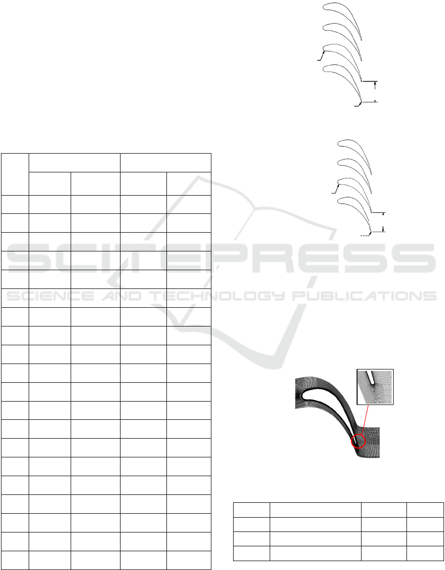
In this research, blade spacing variations were
carried out by increasing and decreasing space from
the original size. The blade spacing variations were
91.74 mm and 70.5 mm.
Figure 1: Blade Geometry with Blade Spacing 91.74 mm.
Figure 2: Blade Geometry with Blade Spacing 70.5 mm.
2.2 Meshing
In this study, meshing was carried out using ICEM
CFD. We want to analyze the wall blade, and the
mesh is reduced to get better results. The local mesh
used in this study is sizing. The meshing chosen for
this study resulted in 45481 elements and 46280
nodes with a minimum skewness of 0.3.
Figure 3: Meshing.
Table 2: Boundary Condition.
No. Description Value Unit
1 Pressure Inlet 89 kPa
2 Pressure Outlet 39 kPa
3 Temperature Inlet 100 ⁰C
R1.15 mm
R10.55
mm
91.74 mm
R10.55
70.5 mm
R1.15
Numerical Study of Outlet Pressure on the Condensing Flow from Steam Turbine Blade with Blade Spacing Variation
315

2.3 Processing
This stage relates to determining the boundary
conditions in a CFD simulation. The wet steam
approach has been used for multiphase modeling, and
the k- ω SSt is used in the viscous model, while the
density-based and steady-state are used for the
solution setup in the solver model.
2.4 Equation
The condensation occurs due to a decrease in pressure
below saturation until the vapor changes from gas to
liquid form.
𝛽=
=
(
)
(1)
𝛽=𝑙𝑖𝑞𝑢𝑖𝑑 𝑚𝑎𝑠𝑠 𝑓𝑟𝑎𝑐𝑡𝑖𝑜𝑛
𝑚
=𝑚𝑎𝑠𝑠𝑎 𝑙𝑖𝑞𝑢𝑖𝑑
𝑚
=𝑚𝑎𝑠𝑠𝑎 𝑣𝑎𝑝𝑜𝑟
𝛼
=𝑣𝑜𝑙𝑢𝑚𝑒 𝑓𝑟𝑎𝑐𝑡𝑖𝑜𝑛 𝑙𝑖𝑞𝑢𝑖𝑑
𝜌
=𝑑𝑒𝑛𝑠𝑖𝑡𝑎𝑠 𝑣𝑎𝑝𝑜𝑟
𝜌
=𝑑𝑒𝑛𝑠𝑖𝑡𝑎𝑠 𝑙𝑖𝑞𝑢𝑖𝑑
The condensation process begins with a
nucleation process with tiny water droplets due to
decreased pressure and temperature. The water
droplets can enlarge as in classical nucleation theory,
or the water droplets can return to steam.
𝐽=
𝑒
∗
(2)
J = Nucleation rate
𝑙
𝑚
𝑠
M = Water mass molecul (kg)
𝑘
= Boltzman constanta
𝑇
= Steam temperature (K)
𝜌
= Steam density
𝑘𝑔
𝑚
𝜌
= Liquid density
𝑘𝑔
𝑚
𝑞
= Condensation Coefficient
𝜎 = Surface tension
𝑁
𝑚
𝜃 = Correction factor non-isotermal
Critical radius of droplet:
𝑟
∗
=
(3)
r = Droplet radius (m)
𝜎 = Liquid surface tension
𝑁
𝑚
R = Gas coefficient
𝐽
𝑘𝑔𝐾
𝜌
= Liquid density
𝑘𝑔
𝑚
T = Temperature (K)
Condensation also affects turbine efficiency. The
amount of condensation can cause a decrease in
efficiency and erosion.
𝜂
=
,
(4)
ℎ
=𝑒𝑛𝑡𝑎𝑙𝑝𝑖 𝑝𝑎𝑑𝑎 𝑠𝑖𝑠𝑖 𝑖𝑛𝑙𝑒𝑡
ℎ
=𝑒𝑛𝑡𝑎𝑙𝑝𝑖 𝑝𝑎𝑑𝑎 𝑠𝑖𝑠𝑖 𝑜𝑢𝑡𝑙𝑒𝑡
ℎ
,
=𝑒𝑛𝑡𝑎𝑙𝑝𝑖 𝑖𝑠𝑠𝑒𝑛𝑡𝑟𝑜𝑝𝑖𝑠 𝑝𝑎𝑑𝑎 𝑠𝑖𝑠𝑖 𝑠𝑡𝑎𝑡𝑜𝑟
𝜂
=𝑒𝑓𝑖𝑠𝑖𝑒𝑛𝑠𝑖 𝑖𝑠𝑒𝑛𝑡𝑟𝑜𝑝𝑖𝑠
3 RESULT AND DISCUSSION
3.1 Grid Independent
The independent grid in this research has been done
by meshing periodically to get the meshing with the
slightest possible error.
Table 3: Mesh Variation.
Number of
Elements
Type
Average
of Static
Pressure
Error
Mesh
33616 A 65176.80 -
41161 B 64943.81 0.1291
45481 C 64001.76 1.4595
58998 D 64023.91 0.0346
60248 E 64026.26 0.0037
There are five mesh variations mesh A with 33616
cells, mesh B with 41161 cells, mesh C with 45481
cells, mesh D with 58998 cells, and mesh E with
60248 cells. The results show that the mesh variation
C has a static pressure starting to be constant.
Compared to the mesh variations, D and E variation
C has the least number of cells, so that the simulation
will be efficient.
iCAST-ES 2021 - International Conference on Applied Science and Technology on Engineering Science
316
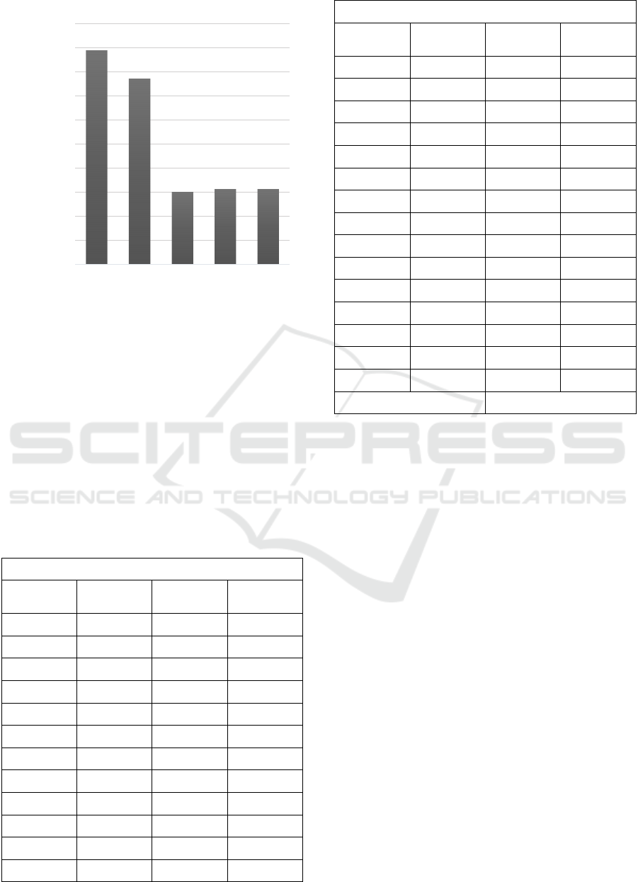
Figure 4: Result of Mesh Independent.
3.2 Validation
Validation using a mesh with variation C has several
elements measuring 45481 with an average statistical
pressure of 64001.76423 Pa. This value is then
compared with the statistical pressure value on the
quoted paper to calculate the error value. The
numerical study is valid if the error is below 3%, and
in Table 4, it is shown that the average error obtained
is 2.9%, so that the simulation in this research is valid.
Table 4: Validation of Static Pressure.
Pressure Side
X
Experiment
(Pa)
Simulation
(Pa)
Error (%)
0.10563 79131.3 79461 0.416649
0.11623 76537.4 76708.7 0.354931
0.12624 72767.3 73694.4 1.274061
0.13557 70497.3 70893.8 0.562433
0.14001 68161.1 69764.9 2.352955
0.14422 67068.2 68689.7 2.417688
0.14825 66396.5 67727.5 2.004624
0.15205 66573.9 67497.8 1.387781
0.15566 66396.5 67015..4 0.932127
0.15908 65508.5 66472.1 1.470954
0.16236 64718.5 65631.6 1.410879
0.16545 63417.8 64284.7 1.366966
Suction Side
X
Experiment
(Pa)
Simulation
(Pa)
Error (%)
0.08121 71100.2 71579.2 0.673697
0.09636 66296.7 67192.3 1.350897
0.10968 60392 61479.5 1.800735
0.12074 57260.1 59292.1 3.548719
0.1295 60608.2 61494.4 1.462178
0.13749 58726 59813.4 1.85165
0.14497 53188.3 53188.3 0
0.14852 47504.6 47504.6 0
0.15191 42063.2 46522.3 10.60095
0.15519 48070 45783.6 4.756397
0.15829 45328.2 40732.1 10.1396
0.16128 42593 38080.2 10.59517
0.1641 38804.2 35829.5 7.665923
0.1668 36061.8 34476.5 4.396065
0.16936 34044.1 32705.1 3.933134
Average of error 2.915821
3.3 The Effect of Blade Spacing
Variations
Condensation occurs when the vapor goes through the
expansion process so that the static pressure drops
below the saturation pressure, which causes a phase
change from the vapor phase to the liquid phase
(Nagib Elmekawy & Ali, 2020).
The value of static pressure on the variation of the
blade spacing P = 91.74 mm, and P = 70.5 mm is
shown in Fig. 4. Static pressure contours show that
changes in blade distance affect the distribution of
static pressure, especially in the trailing edge area.
The static pressure contour shows that the pressure at
the inlet blade is greater than the outlet pressure. The
lowest pressure drop value was obtained in the most
significant variation of blade distance P = 91.74 mm,
while the slightest variation of blade distance P = 70.5
mm had the highest pressure drop. The smaller the
blade distance, the smaller the cross-sectional area of
the flow and increases the rate of steam expansion so
that there is a greater chance of condensation.
63400
63600
63800
64000
64200
64400
64600
64800
65000
65200
65400
33616 41161 45481 58998 60248
Average of Static Pressure
Number of Elements
Mesh Variations
Numerical Study of Outlet Pressure on the Condensing Flow from Steam Turbine Blade with Blade Spacing Variation
317
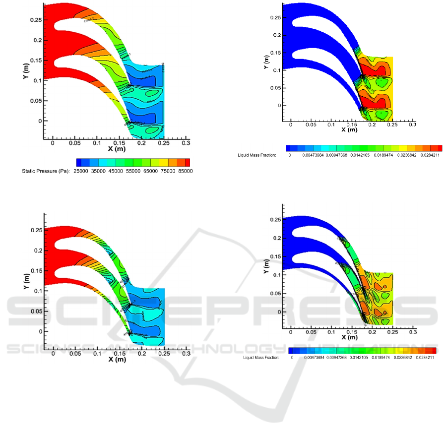
Figure 5: Contour of static pressure (Pa) for blade spacing
P = 91.74 mm.
Figure 6: Contour of static pressure (Pa) for blade spacing
P = 70.5 mm.
The liquid mass fraction contour describes the
state of the vapor in the gap between the blades. The
liquid fraction in Fig. 5 is found around the trailing
edge. It is because the rate of steam expansion in the
area has the highest value. The contours of the liquid
mass fraction for various blade spacing variations are
P = 91.74 mm, and P = 70.5 mm. It can be seen that
the smaller the distance between the blades, the more
liquid fraction is formed. In the variation of the blade
distance, P = 70.5 mm has the most liquid mass
fraction, which is indicated by more areas that have a
fraction value of more than 0, which reflects that
much water is formed compared to other variations.
In addition, as the blade spacing widens, the zone
with a value greater than 0 becomes narrower.
Figure 7: Contour of liquid mass fraction for blade spacing
P = 91.74 mm.
Figure 8: Contour of liquid mass fraction for blade spacing
P = 70.5 mm.
The droplet growth rate is the number of droplets
produced every second. From the droplet growth rate
contours in Fig. 6, it can be seen that variations in
blade distance can affect the speed of droplet
formation in the blade gap. In the variation, P = 91.74
mm has a maximum droplet growth rate of 1212.663
microns/s; at variation, P = 70.5 mm has a maximum
droplet growth rate of 1280.906 microns/s. Then the
variation of the distance P = 91.74 mm, and P = 70.5
mm, it is known that the smaller the distance between
the blades, the higher the droplet formation speed. It
can be seen in the droplet growth rate contour at
variation P = 70.5 mm, which has many red zones,
while at variation P = 91.74 mm has the lowest
droplet growth rate, which is indicated by the minor
red zones. When compared to each variation, the
highest droplet growth was in the P = 70.5 mm
variation with a maximum velocity value of 1280,906
microns/s.
iCAST-ES 2021 - International Conference on Applied Science and Technology on Engineering Science
318
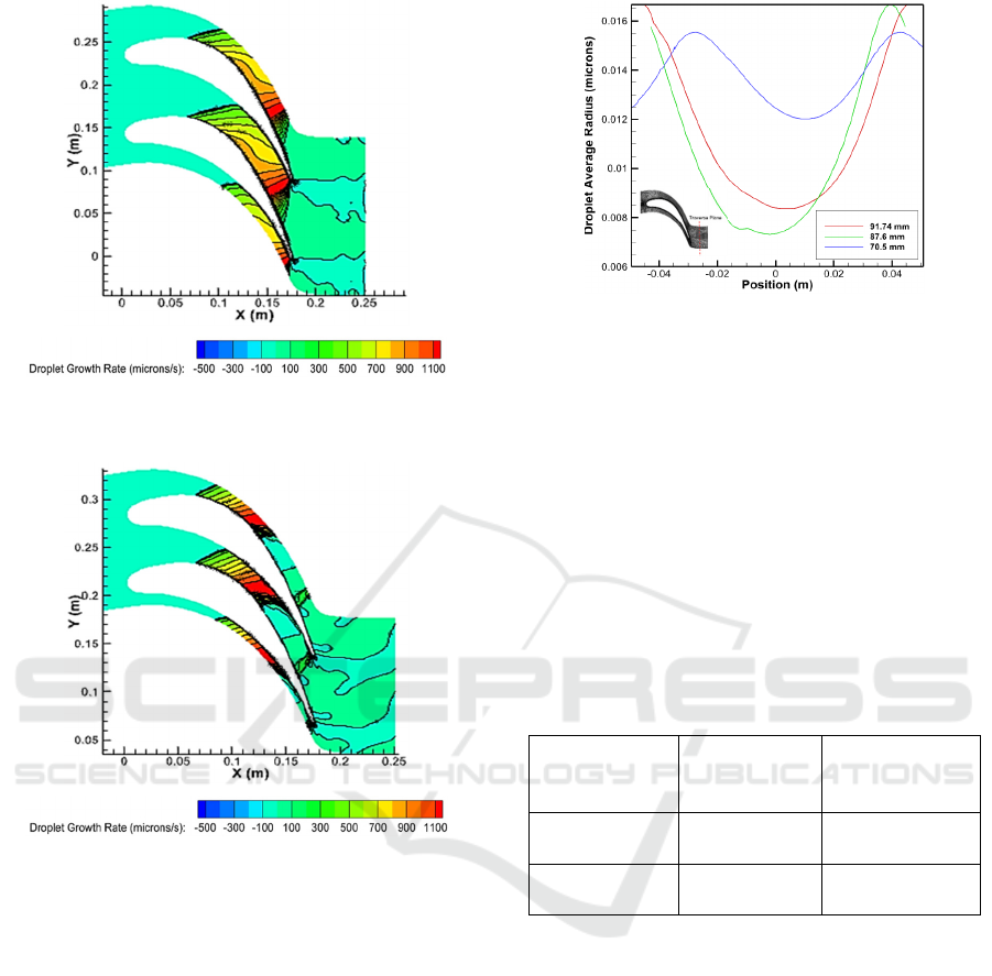
Figure 9: Contour of droplet growth rate (microrns/s) for
blade spacing P = 91.74 mm.
Figure 10: Contour of droplet growth rate (microrns/s) for
blade spacing P = 70.5 mm.
Variations in the distance between blades affect
the droplet radius. In Fig. 7, The variation of P =
91.74 mm has the lowest droplet radius, while the
variation of distance P = 70.5 mm has the largest
droplet radius. It shows that the smaller the distance
between the blades, the greater the droplet growth rate
according to the droplet growth rate contour. When
compared with distance variations, it can be seen that
the smaller the distance between the blade radius
formed, the larger the radius. The 70.5 mm variation
has the most considerable minimum radius value of
0.01 microns. It is because the pressure on the
mainstream blade with a smaller distance will also be
smaller.
Figure 11: Graph of droplet average radius (microrns) for
blade spacing variations.
Table 5 is the result of calculating the isentropic
efficiency of the blade. The calculation of isentropic
efficiency is carried out to determine the effect of the
distance between blades on efficiency. It is known
that the distance between blades can affect isentropic
efficiency. The smaller the distance between the
blades, the smaller the isentropic efficiency of the
blade. At a distance of P = 91.74mm, the highest
efficiency is 88.06 %, and at a distance of P = 70.5
mm, the lowest efficiency is 85.37%. It is caused by
the outlet pressure getting smaller and the smaller
variations in the distance between the blades.
Table 5: Isentropic Efficiency.
Blade
Spacing
Variation
Outlet
Pressure
(kPa)
Isentropic
Efficiency
(%)
P = 91.74 mm 39.25 88.06
P = 70.5 mm 39.07 85.37
4 CONCLUSIONS
The blade stator is simulated by numerical simulation
with Computational Fluid Dynamic (CFD) with
variations in blade distance resulting in the following
main conclusions. Variations in the distance between
blades affect the distribution of static pressure on the
steam flow. The blade with a distance of P = 70.5 mm
has the highest expansion rate because it has the
lowest minimum pressure of 13703.65 Pa and
variations in the distance between blades affect the
formation of condensation, which can be seen from
the contours of the liquid mass fraction. The blade
with the smallest distance P = 70.5 mm has a liquid
mass fraction zone and has a widest value of more
than 0, which means more condensate is formed also
Numerical Study of Outlet Pressure on the Condensing Flow from Steam Turbine Blade with Blade Spacing Variation
319

can be seen from the droplet growth contour. The
blade with the smallest distance P = 70.5 mm has the
highest droplet formation speed of 1280.906
microns/s. The average droplet radius graph shows
variations with the smallest distance P = 70.5 mm
having the largest droplet radius with a minimum of
0.01 microns and the isentropic efficiency table
shows the variation with the lowest efficiency at
variation P = 70.5 mm by 85.37%he blade spacing
variation affects the distribution of static pressure on
the steam flow, where the blade with the smallest
distance P = 70.5 mm has the highest expansion rate
compared to other variations.
ACKNOWLEDGEMENTS
The authors acknowledge to PENS (Politeknik
Elektronika Negeri Surabaya) for support this
research.
REFERENCES
Buckley, J. R. (2003). A Study of Heterogeneous Nucleation
and Electrostatic Charge in Steam Flows. November.
Cao, L., Wang, J., Luo, H., Si, H., & Yang, R. (2020).
Distribution of condensation droplets in the last stage
of steam turbine under small flow rate condition.
Applied Thermal Engineering, 181(September),
116021. https://doi.org/10.1016/j.applthermaleng.20
20.116021
Diana, L., Safitra, A. G., & Muhammad, G. (2019).
Numerical Investigation of Airflow in a Trapezoidal
Solar Air Heater Channel. IES 2019 - International
Electronics Symposium: The Role of Techno-
Intelligence in Creating an Open Energy System
Towards Energy Democracy, Proceedings, 248–253.
https://doi.org/10.1109/ELECSYM.2019.8901524
Jensen, K. R., Fojan, P., Jensen, R. L., & Gurevich, L.
(2014). Water condensation: A multiscale
phenomenon. Journal of Nanoscience and
Nanotechnology, 14(2), 1859–1871. https://doi.org/
10.1166/jnn.2014.9108
Jonas, O., & Machemer, L. (2008). Steam Turbine
Corrosion and Deposits Problems and Solutions.
Thirty-Seventh Turbomachinery Symposium, 211–228.
Manushin, E. A. (2011). Steam Turbine. A-to-Z Guide to
Thermodynamics, Heat and Mass Transfer, and Fluids
Engineering.
https://doi.org/10.1615/atoz.s.steam_turbine
Nagib Elmekawy, A. M., & Ali, M. E. H. H. (2020).
Computational modeling of non-equilibrium
condensing steam flows in low-pressure steam turbines.
Results in Engineering, 5, 100065. https://doi.org/10.10
16/j.rineng.2019.100065
Syahputra, R., Wahyu Nugroho, A., Purwanto, K., &
Mujaahid, F. (2019). Dynamic performance of
synchronous generator in steam power plant.
International Journal of Advanced Computer Science
and Applications, 10(12), 389–396. https://doi.org/
10.14569/ijacsa.2019.0101251
Wood, S. E., Baker, M. B., & Swanson, B. D. (2002).
Instrument for studies of homogeneous and
heterogeneous ice nucleation in free-falling
supercooled water droplets. Review of Scientific
Instruments, 73(11), 3988. https://doi.org/10.1063/
1.1511796
iCAST-ES 2021 - International Conference on Applied Science and Technology on Engineering Science
320
