Robust Teeth Detection in 3D Dental Scans by Automated Multi-view

Landmarking

Tibor Kub

ık

and Michal

Span

1,2 a

Department of Computer Graphics and Multimedia, Faculty of Information Technology,

Brno University of Technology, Brno, Czech Republic

TESCAN 3DIM, Brno, Czech Republic

Keywords:

Landmark Detection in 3D, Polygonal Meshes, Multi-view Deep Neural Networks, RANSAC, U-Net,

Heatmap Regression, Teeth Detection, Dental Scans.

Abstract:

Landmark detection is frequently an intermediate step in medical data analysis. More and more often, these

data are represented in the form of 3D models. An example is a 3D intraoral scan of dentition used in or-

thodontics, where landmarking is notably challenging due to malocclusion, teeth shift, and frequent teeth

missing. What’s more, in terms of 3D data, the DNN processing comes with high memory and computational

time requirements, which do not meet the needs of clinical applications. We present a robust method for

tooth landmark detection based on a multi-view approach, which transforms the task into a 2D domain, where

the suggested network detects landmarks by heatmap regression from several viewpoints. Additionally, we

propose a post-processing based on Multi-view Conﬁdence and Maximum Heatmap Activation Conﬁdence,

which can robustly determine whether a tooth is missing or not. Experiments have shown that the combination

of Attention U-Net, 100 viewpoints, and RANSAC consensus method is able to detect landmarks with an error

of 0.75 ± 0.96 mm. In addition to the promising accuracy, our method is robust to missing teeth, as it can

correctly detect the presence of teeth in 97.68% cases.

1 INTRODUCTION

The localization of landmarks plays a crucial role in

many tasks related to image analysis in medicine.

Deep learning has demonstrated great success in this

ﬁeld, outperforming conventional machine learning

methods. With the widespread availability of accu-

rate 3D scanning devices, this task has moved into

a 3D domain. This brings us the possibility of in-

creased automation of clinical application tasks that

operate on 3D models, such as in the case of digital

orthodontics.

In terms of direct 3D data processing by neu-

ral networks, a noticeable challenge has emerged as

the size of the input feature vector substantially in-

creases. The time of computation of such deep neu-

ral networks is not suitable for clinical applications

used during treatment planning in digital orthodon-

tics. 3D medical data analysis reckons with an-

other challenge – the limited amount of medical data,

a common struggle in medical image processing.

https://orcid.org/0000-0003-0193-684X

Dentition casts used in digital orthodontics soft-

ware are typically obtained from patients with various

levels of malocclusion and numerous kinds of teeth

shifting. Another challenging problem in this do-

main is the absence of teeth, a common phenomenon

in terms of human dentition. The 3rd Molars (also

known as Wisdom teeth) are worth taking a look at.

Their extraction is one of the most frequent proce-

dures in oral surgery as it eliminates future problems

due to unfavorable orientation (Normando, 2015).

Thus, the method should be robust to such variations.

In this paper, we present a method that consid-

ers the limitation of the dataset size, the need for low

computational time, and the importance of robustness

to missing and shifted teeth. It is based on a multi-

view approach and it uses heatmap regression to pre-

dict landmarks in 2D and the RANSAC consensus

method to robustly propagate the information back

into 3D space. In order to address the problem of es-

timation of landmarks on missing teeth, our method

comprises a post-processing based on a heatmap re-

gression uncertainty analysis combined with the un-

certainty of the multi-view approach.

Kubík, T. and Špan

el, M.

Robust Teeth Detection in 3D Dental Scans by Automated Multi-view Landmarking.

DOI: 10.5220/0010770700003123

In Proceedings of the 15th International Joint Conference on Biomedical Engineering Systems and Technologies (BIOSTEC 2022) - Volume 2: BIOIMAGING, pages 24-34

ISBN: 978-989-758-552-4; ISSN: 2184-4305

0.0

2.0 mm

4.0 mm

6.0 mm

8.0 mm

10.0+ m

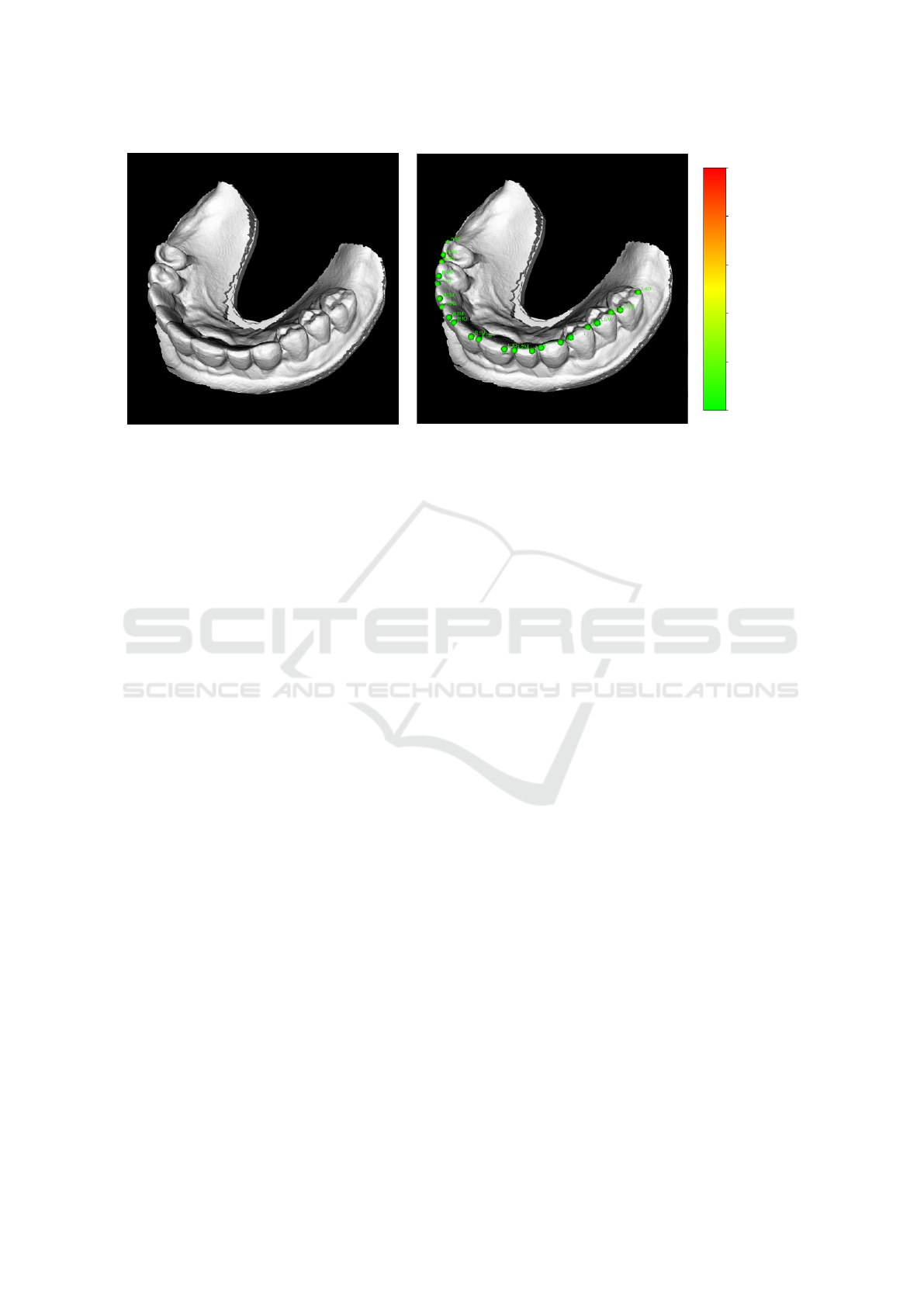
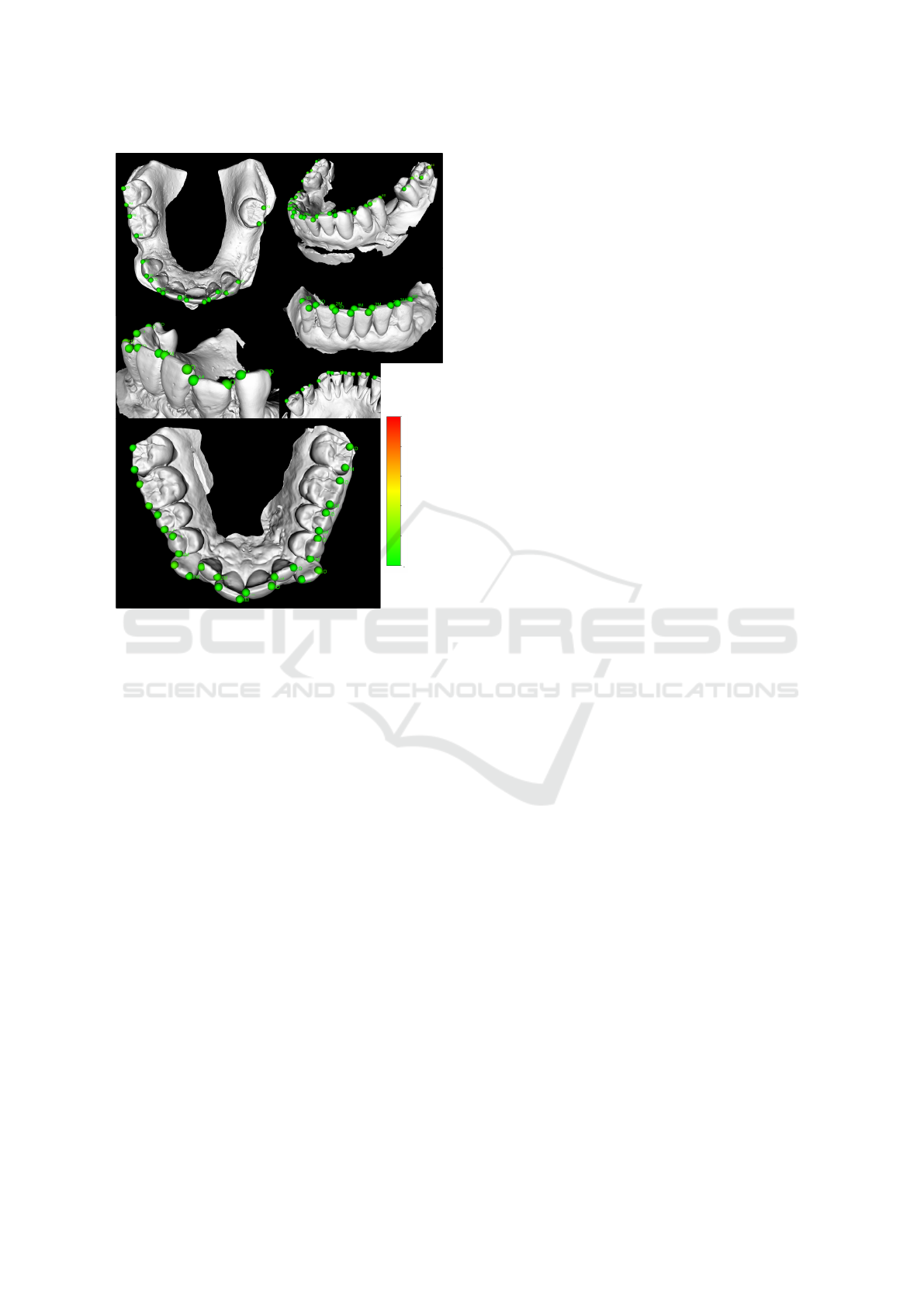
(a) Input polygonal mesh (b) Detected landmarks with our method

Figure 1: An example of a 3D scan of dentition (a) and appropriate detected landmarks (b). Our method automatically detects

two landmarks on each tooth – mesial and distal. This type of landmarks is important in orthodontics, as it deﬁnes the rotation

of teeth from anatomically perfect arrangement. Whatsmore, the method correctly detects whether a tooth is missing or not.

Conducted experiments have shown that the pro-

posed method can detect orthodontics landmarks on

surface models with an error of 0.75 ± 0.96 mm

while 98.07% of detected landmarks achieve an er-

ror less than 2 mm. As for the robustness to missing

teeth, our method’s post-processing correctly detects

missing teeth in 97.68% of cases.

2 CURRENT APPROACHES TO

LANDMARKING

Early studies in this area relied on conventional ma-

chine learning approaches. Hough forests were used

for landmark detection. Authors in (Donner et al.,

2013) combined regression and classiﬁcation, which

brought better results comparing to both a single

voxel’s classiﬁcation and classiﬁcation of the vol-

ume of interest. As convolutional neural networks

(CNNs) gained in popularity, an increasing number

of scientiﬁc papers concerning their usage in land-

mark detection emerged. Some of these methods de-

tected the landmark position directly by regressing

its x and y coordinates. For example, in (Sun et al.,

2013), the authors adopted cascaded convolutional

neural networks for facial point detection. Another

study (Lv et al., 2017) proposed a regression in a two-

stage manner, still locating landmarks directly.

2.1 Heatmaps in Landmarking

Over time, extensive literature has developed on land-

marking by heatmap regression. The authors in (Pﬁs-

ter et al., 2015) worked on a model that regresses hu-

man joint positions. Instead of directly regressing the

(x, y) joint position, they regressed a joint position’s

heatmap. During the training, the ground truth labels

are transformed into heatmaps by placing a Gaussian

with ﬁxed variance at each joint coordinate.

On top of the appliance of spatial fusion layers and

optical ﬂow, they discussed the beneﬁts of regress-

ing a heatmap rather than (x, y) coordinates directly.

They concluded that the beneﬁts are twofold: (i) the

process of network training can be visualized in such

a way that one can understand the network learning

failures, and (ii) the network output can acquire conﬁ-

dence at multiple spatial locations. The incorrect ones

are slowly suppressed later in the training process. In

contrast, regressing the (x, y) coordinates directly, the

network would have a lower loss only if it predicts

the coordinate correctly, even if it was “growing con-

ﬁdence” in the correct position. Concerning these,

such an approach outperformed direct coordinate re-

gression and became a standard way of landmark de-

tection in 2D images.

This approach seemed alluring for people in the

medical image processing community. Inspired by

this method, authors in (Payer et al., 2016) pre-

sented multiple architectures that detect keypoints in

X-Ray images of hands and 3D hand MR scans. They

afﬁrmed that by regressing heatmaps, it is possible

to achieve state-of-the-art localization performance in

2D and 3D domains while dealing with medical data

shortage.

Robust Teeth Detection in 3D Dental Scans by Automated Multi-view Landmarking

2.2 Processing of 3D Data by Neural

Networks

Although the extension of deep neural network op-

erations such as convolution from 2D to 3D domain

seems natural, the additional computational complex-

ity introduces notable challenges. Having volumet-

ric data (for example, voxel models) or 3D surface

data (for example, represented as polygon meshes) as

an input to deep neural networks has a considerable

drawback in computational time and memory require-

ments.

An alternative way of 3D data processing by neu-

ral networks is the multi-view approach. Obtaining

state-of-the-art results on 3D classiﬁcation, authors

in (Su et al., 2015) presented the multi-view CNN

idea. It is relatively straightforward and consists of

three main steps:

1. Render a 3D shape into several images using vary-

ing camera extrinsics.

2. Extract features from each acquired view.

3. Process features from different viewpoints in

a way suitable for a given task. In (Su et al., 2015),

a pooling layer followed by fully connected layers

was used to get class predictions.

The multi-view approach was later on used to

identify feature points on facial surfaces (Paulsen

et al., 2018). The authors discussed multiple geom-

etry derivatives and experimented with their combi-

nations to bring state-of-the-art results in feature point

detection on facial 3D scans while decreasing the pro-

hibitive GPU memory requirements needed for true

3D processing. Additionally, they proposed a con-

sensus method to ﬁnd the ﬁnal estimate, which com-

bines the least-squares ﬁt and RANdom SAmple Con-

sensus (RANSAC) (Fischler and Bolles, 1981). For

each landmark, N rays in 3D space are the outputs of

the proposed method.

Based on Graph Neural Networks (GNNs), au-

thors in (Sun et al., 2020) presented coupled 3D seg-

mentation for annotation of individual teeth and gin-

giva. Their network produces a dense correspondence

that helps to accurately locate individual orthodon-

tics landmarks on teeth crowns. Another recent work

in landmark localization on dental mesh models was

presented by authors in (Wu et al., 2021). They in-

troduced a two-stage framework based on mesh deep

learning (TS-MDL) for joint tooth labeling and land-

mark identiﬁcation. To accurately detect tooth land-

marks, they designed a modiﬁed PointNet (Qi et al.,

2017) to learn the heatmaps encoding landmark loca-

tions.

We have developed a generic method based on the

current approaches in landmarking to solve a variety

of problems that arose from the medical character of

the dataset:

• the method should be robust to missing teeth,

• tens of cases should be sufﬁcient to train the net-

work,

• and the speed of the inference should be fast

enough to be used in a clinical application.

Especially valuable is the introduced post-

processing based on heatmap regression uncertainty

analysis and analysis of the uncertainty of the multi-

view approach. It ensures that our method cor-

rectly detects landmark presence without any addi-

tional computations. This is inevitable for orthodontic

ﬂow as it robustly detects teeth presence even in chal-

lenging cases (e.g., already discussed 3rd molars).

This aspect was not discussed in recent works that

deal with orthodontics landmarks on teeth crowns.

In addition to the post-processing and the method

itself, this paper presents valuable comparisons and

experiments on various factors that impact the efﬁ-

ciency of alternative variations of the method:

• rendering type of the processed 3D object to be

used as an input (depth map, geometry or combi-

nation of both),

• comparison of several network designs (U-Net,

Attention U-Net, and Nested U-Net),

• the analysis of the results of two consensus meth-

ods: a method that calculates the centroid of mul-

tiple predictions and a geometric method based on

the RANSAC algorithm and least-squares ﬁt,

• and the analysis of the correlation between the

number of viewpoints and the method accuracy.

3 DATASET OF 3D DENTAL

SCANS AND LANDMARKS IN

THIS STUDY

Our method was trained and evaluated on a dataset of

337 3D dental scans of human dentition represented

as polygon meshes. The dataset contains cases of

both maxillary and mandibular dentition. Since all

dentition scans were anonymized, it is not possible to

undertake complex analysis of patients’ age or ethnic-

ity. Therefore, the data analysis was empirical and fo-

cused on aspects such as the frequency of absence of

teeth, the rate of healthy dentition, and dentition with

malocclusion and shifted teeth. Concerning these as-

pects, our data reﬂect real orthodontics patients since

BIOIMAGING 2022 - 9th International Conference on Bioimaging

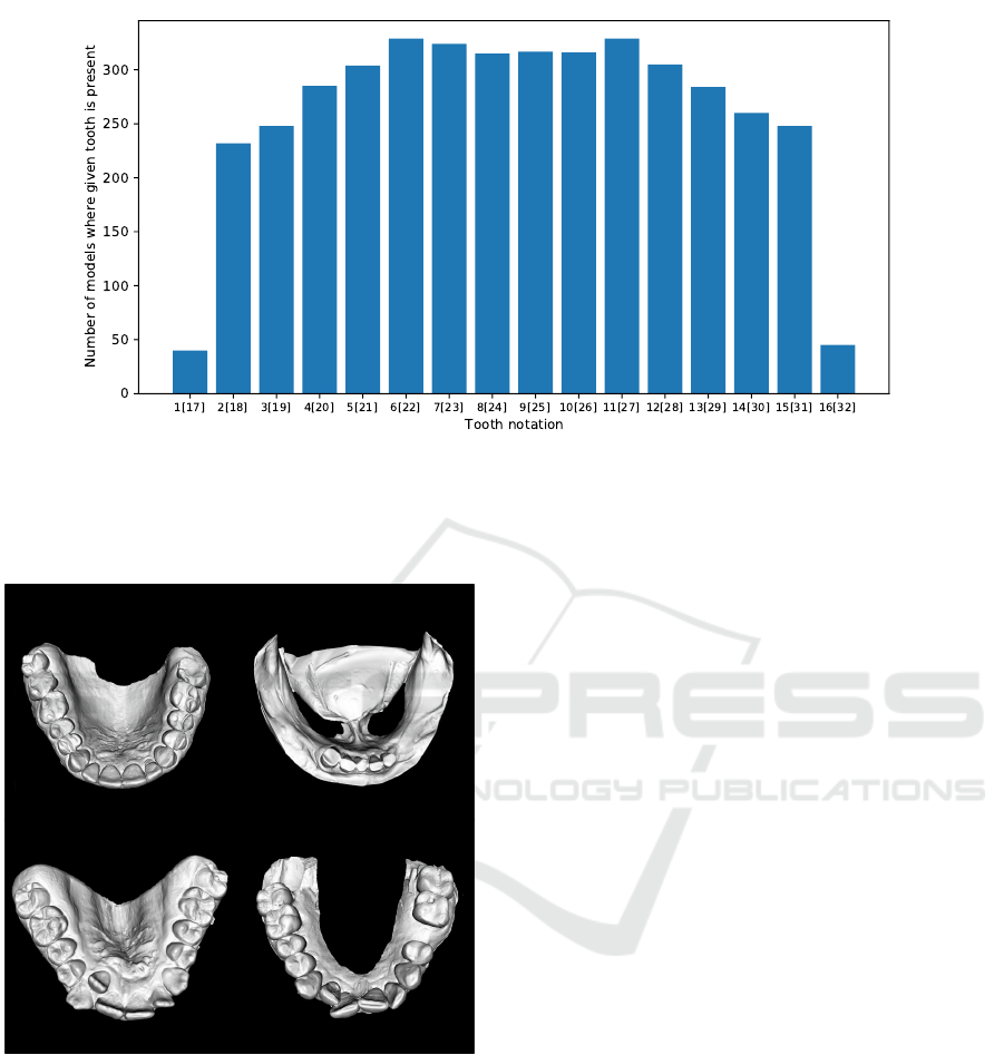
Figure 2: Distribution of casts where given tooth is present on the dentition. For example, out of 337 scanned dentition from

the dataset, less than 50 cases contain either left or right 3rd molar. This distribution reﬂects the reality, as 3rd molars are

often extracted (Normando, 2015). On the other hand, canines and incisors are present in the vast majority of models. Please

note that the Universal Numbering System is used to refer teeth. Also note that teeth 1 and 17 are considered as the same

category, likewise to the rest of the teeth.

Figure 3: Examples of dental casts within the dataset. Data

were collected from orthodontics patients, so patients usu-

ally suffer from different kinds of malocclusion, as depicted

on the bottom examples.

the diversity of data is signiﬁcant, which is essential

for the algorithm’s robustness. Figure 3 depicts the

variety of dentitions in our dataset. The frequency

of missing teeth conﬁrms the diversity in orthodon-

tics cases as well. Figure 2 shows the number of

cases where individual teeth are not missing within

the dataset. Landmarks used in this study address the

digital orthodontics ﬂow in the existing planning soft-

ware. These landmarks deﬁne the mesial and distal

location of each tooth. They are placed on the oc-

clusal surface of molars and premolars and the incisal

surface on canines and incisors, as close to the cheek-

facing surfaces as possible. In other words, 32 land-

marks must be placed on one arch in case of full den-

tition, two for each tooth. Ground truth positions of

landmarks were annotated by one person only.

4 PROPOSED SOLUTION FOR

ORTHODONTICS LANDMARK

DETECTION

An outline of our method can be found in Figure 4.

Prior to each evaluation, there is a precondition to

align the evaluated mesh so the occlusal surfaces face

the camera. Afterward, following the multi-view ap-

proach, the model is observed from various camera

extrinsics. We used uniformly distributed positions

of the camera with a maximal angle of ± 30 degrees

from the initial aligned position.

Network Inputs and Outputs

Images in the form of depth maps and direct rendering

of the geometry are used as the inputs to the neural

network.

From each acquired view, features are extracted

and processed in the heatmap regression manner. In

a similar way as in (Pﬁster et al., 2015), during train-

ing, the input example is denoted as a tuple (X, y),

Robust Teeth Detection in 3D Dental Scans by Automated Multi-view Landmarking

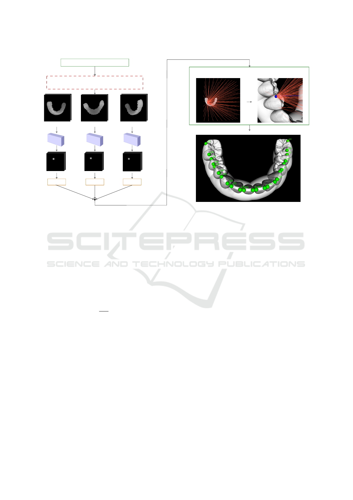
Multi-view rendering

3D scan in STL format

... View 1 < n < N ... View N

CNN

... ...

...

}

...

}

...

}

... ...

2D ↦ 3D

Predictions: points/rays

Consensus method

Octree based-search division

Result: predicted landmarks in 3-space

For each landmark

}

Depth map

+ geometry

... ...

Figure 4: Outline of the proposed method for orthodontics landmark detection. Following the multi-view approach, input 3D

model is observed from various viewports and sent to the CNNs to produce heatmaps. Landmark screen coordinates are ex-

tracted from obtained heatmaps and further processed by the consensus method, which produces ﬁnal estimates. Additionally,

the maximum value in the activation map, together with the output of the consensus method, are used to detect tooth presence

during post-processing.

where X is the 2-channel input and y stands for the

coordinates of 32 landmarks located in input X. Fur-

thermore, the training data are denoted as N = {X, y}

and the network regressor as φ. Then, the training ob-

jective is the estimation of the network weights λ:

argmin

∑

(X,y)∈N

∑

i, j,k

) − φ

i, j,k

(X,λ)k

(1)

where G

i, j,k

) =

2πσ

−[(y

−i)

+(y

− j)

]/2σ

a Gaussian centered at landmark y

with ﬁxed σ.

Using this approach, the last convolutional layer’s

output is a heatmap represented as a ﬁxed-size

i × j × 32-dimensional matrix. This implies that the

the predicted results are 32 channels (as we intend to

predict 32 landmarks in our data).

Interpretation of Heatmap Regression Output in

Terms of 3D Data

The predicted 2D heatmap can be interpreted as the

landmark’s screen coordinate (in IR

) position (x, y).

Each output channel contains a heatmap with a Gaus-

sian representing the probability of a given land-

mark’s screen coordinate in each pixel. Thus, the re-

sulting screen coordinate must be extracted from the

predicted heatmap by ﬁnding coordinates of the peak

value. It is indispensable to propagate the coordinates

into a world coordinate system IR

and ﬁnd a ﬁnal es-

timate by combining outputs from all camera views.

With the known position of the center of projec-

tion, the prediction for a single view of one landmark

can be interpreted as (i) a ray deﬁned by the origin in

the corresponding center of projection and the point

on the view plane at detected screen coordinates or

(ii) simply a point in the 3D scene, i.e. the converted

display coordinate into 3D space.

Consensus Methods

These individual predictions are combined in a con-

sensus method, which is a standard post-processing

step in the multi-view approach. Based on the maxi-

mum value in the activation map, only certain predic-

tions above the experimentally determined threshold

are sent to the consensus method. Certainty analy-

sis will be discussed later in this work. If the pre-

dictions are interpreted as rays, the consensus method

combines the RANSAC algorithm to eliminate partial

predictions classiﬁed as outliers with the least-squares

ﬁt.

To achieve this, we deﬁned each ray by its origin

and a unit direction vector n

, similarly as (Paulsen

et al., 2018). Then, the sum of squared distances from

BIOIMAGING 2022 - 9th International Conference on Bioimaging

a point p is calculated as follows:

∑

[(p − a

)

(p − a

) − [(p − a

)

]

]. (2)

It is necessary to differentiate this equation with re-

spect to p. It brings the solution p = S

C, where

denotes the pseudo-inverse of S. In this case,

S =

∑

− I) and C =

∑

− I)a

The RANSAC procedure initially estimates the value

of p by three randomly chosen rays. The residual is

computed as the sum of squared distances (see Equa-

tion 2) from p to the included rays, and the iterative

RANSAC algorithm then performs I iterations. In

each of these iterations, the number of inliers and out-

liers is calculated, respecting a predeﬁned threshold τ.

This is a minimizing task that ﬁnds a point in IR

with

the shortest distance to all remaining lines.

This method can be interchanged with a more sta-

tistical approach that is less computationally demand-

ing, and it simply ﬁnds the mean position of the pre-

dicted points. Let’s consider N as the number of views

used in the multi-view approach. Let’s also interpret

the single-view evaluation output as a point on the tar-

get polygonal model. With N views, the ﬁnal out-

put P is a single point in IR

and is calculated from

N points as a mean value of these points.

Finding Closest Point on Mesh Surface

These methods ﬁnd the estimation among multiple

predictions, but do not guarantee that the predicted

landmark is placed on the surface of the evaluated

polygonal model. Thus, the last necessary step is to

ﬁnd the closest point on the surface of the polygonal

model. An octree data structure contains a recursively

subdivided target polygonal model. The center of the

closest face on the surface of the polygonal model to

the consensus output is considered the ﬁnal estimate.

4.1 Post-processing for Classiﬁcation of

Teeth Presence

As discussed in previous sections, assuming that the

evaluated 3D scan represents full dentition would be

loose. Therefore, apart from the accurate placement

of the present landmarks, our post-processing con-

tains an analysis of the presence of each tooth (i. e., of

corresponding couple of landmarks). This is in fact

a binary classiﬁcation task, whose result is based on

two uncertainty hypotheses:

• Like in (Drevick

y and Kodym, 2020), the net-

work is trained to regress heatmaps with the am-

plitude of 1. Then, the fundamental assumption

100

120

Peak value: 0.012, GT Presence: False

0.000

0.002

0.004

0.006

0.008

0.010

0.012

100

120

Peak value: 0.7838, GT Presence: True

0.0

0.1

0.2

0.3

0.4

0.5

0.6

0.7

Figure 5: Examples of predicted heatmaps and analysis of

the uncertainty. The top picture illustrates an example of

a prediction with low peak value (0.012). Referencing to

corresponding ground truth, this landmark is not present on

the surface of the polygonal model. The bottom picture, on

the other hand, shows the opposite situation. According to

the ground truth, the peak value is relatively high, and this

landmark is really present on evaluated polygon mesh. Note

that the maximal amplitude value in a heatmap is 1.

is that during the inference, the certainty is mea-

sured by the maximum value in the activation

map, with a proportional increase to the network’s

conﬁdence (Maximum Heatmap Activation Conﬁ-

dence). See Figure 5 for an example.

• The RANSAC consensus method robustly esti-

mates the landmark position by eliminating out-

lier predictions. Thus, the proportion of inliers

and outliers is another valuable output of this con-

sensus method, assuming the number of inliers is

proportional to the overall conﬁdence (Multi-view

Conﬁdence).

These assumptions result in a threshold value,

which combines the Maximum Heatmap Activation

Conﬁdence and Multi-view Conﬁdence, both in a unit

range and equally weighed. The optimal threshold

value can be determined by standard approaches for

Robust Teeth Detection in 3D Dental Scans by Automated Multi-view Landmarking

a binary classiﬁer, as an example by the ROC curve.

This goes to show that such post-processing delivers

vital data for classiﬁcation of landmarks presence by

self-evaluation, i. e., no additional computations or

network evaluations are needed to obtain such infor-

mation. Having the requirement of low computational

time in mind, this is more than eligible.

5 EXPERIMENTS AND RESULTS

To ﬁnd the best possible results, we experimen-

tally investigated and compared several parts of the

method:

• Architecture Design: we compared the U-Net ar-

chitecture with two of its offshoots: the Attention

U-Net and the Nested U-Net.

• Consensus Methods: a comparison of RANSAC

consensus method with centroid calculation is

presented.

• Viewpoint Numbers for the Multi-view Ap-

proach: we analysed whether the increase of

viewpoint number has an impact on the method

accuracy. We experimented with 1, 9, 25, and

100 views.

• CNN Inputs: depth map, direct geometry ren-

dering and its combination (2-channel input) were

compared.

All metrics are measured in physical units (mm)

since the end clinical application is related to physical

units.

5.1 Training Procedure

The input to the neural network is either a single-

channel depth map, single-channel image of the ren-

dered geometry, or two-channel combination of both,

depending on experiment. In all cases, the size of

input was set to 128 × 128. The training procedure

ran on an NVIDIA GeForce RTX 2060 with 6 GB of

memory.

The dataset of 337 dental scans was divided into

a set of 247 cases used for training and a test set of

90 cases. Furthermore, the training set was split in

the ratio of approximately 4:1 into a training and val-

idation set, respectively.

Following augmentation techniques were applied

to both, the 2D input(s) and the ground truth

heatmaps:

• Scale: in the range [0.90, 1.10],

• Rotation: in the range [−30, 30] degrees,

• Translation: in the range [−10 px, 10 px] and ap-

plied in both vertical and horizontal directions.

Training Parameters and Loss Function

Networks were trained using the Adam optimizer

with the weight decay set to 10

−3

. The learning rate

was initially set to 10

−3

. Its value was dynamically

reduced using learning rate scheduler. The learning

rate was reduced by a factor of 0.5 every time the

value of validation loss has not improved for 5 con-

secutive epochs. The validation loss was monitored

for the early stopping. If the validation loss value

did not improve for more than 20 consecutive epochs,

the training was stopped. To reduce the memory re-

quirements during training, the automatic mixed pre-

cision was used. The batch size was set to 32. To

train the models on a regression problem, the Root

Mean Square Error (RMSE) loss was used.

5.2 Overall Results

The main focus of the experiments was to ﬁnd the

best setup of the method. Overall results are sum-

marized in Table 1. Our results show that the ac-

quired accuracy is mostly inﬂuenced by the consensus

method, where RANSAC outperforms the Centroid

by a large margin in all setups. As for the used ar-

chitecture, the overall results show that the Attention

U-Net performs slightly better than the rest. Combi-

nation of depth maps and geometry renders impacts

the results in a positive way as well. See Figure 7 for

box plots of radial errors of individual detected land-

marks. The Attention U-Net has 526 534 trainable pa-

rameters and inference takes 4 seconds on average on

Intel Core i7-8750H CPU @ 2.20 GHz with 6 cores

(using 25 views).

When comparing our results to the framework

from (Wu et al., 2021), speciﬁcally with their best-

performing strategy, 2-stage iMeshSegNet+PointNet-

Reg. In terms of accuracy, they achieve a slightly

better error of 0.623 ± 0.718 mm. Their approach

slightly outperforms ours (in best-performing con-

ﬁguration, 0.75 ± 0.96 mm), but it is necessary

to keep in mind several factors. As a matter of

fact, their dataset consists of 36 samples. Such rel-

atively small number should be increased to ensure

the method’s robustness to the large variability of or-

thodontic cases. Our dataset is more challenging and

consists of problematic cases with severe teeth shift-

ings and of many cases with missing teeth. In addi-

tion, they detect landmarks only on 10 teeth, exclud-

ing, for example, very problematic 3rd molars. Thus,

for a fair comparison, it would be vital to benchmark

BIOIMAGING 2022 - 9th International Conference on Bioimaging

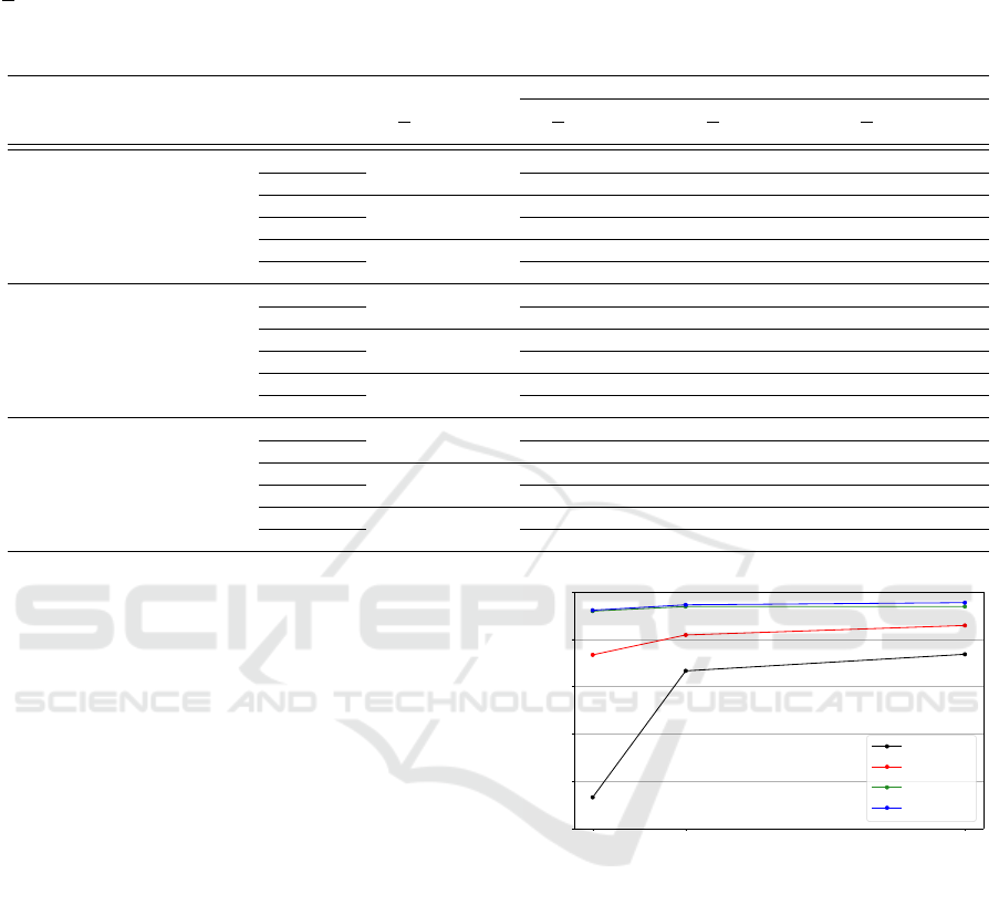
Table 1: Overall results of the individual networks with different multi-view settings. Table compares the system performance

with different combinations of architectures, network inputs, consensus methods, and number of viewpoints. A combination

of the Attention U-Net architecture, the RANSAC consensus method, and 100 rendered views achieves the best performance.

R stands for the mean radial error, and SD stands for standard deviation. Values are calculated from all predicted landmarks on

dental scans from the test dataset and measured in millimeters (mm). All values are measured on networks with class-balanced

loss. Please note that the alignment of evaluated 3D scans inﬂuence the measured values.

Single-view

Multi-view

Architecture & N = 9 N = 25 N = 100

consensus method R SD R SD R SD R SD

BN U-Net (Depth)

Centroid

2.24 4.02

2.00 2.37 1.74 2.33 1.80 1.96

RANSAC 1.24 2.86 1.02 3.75 1.01 4.28

BN U-Net (Geom)

Centroid

2.13 4.41

2.03 3.14 1.69 2.21 1.67 2.41

RANSAC 1.20 3.01 1.17 2.16 1.06 2.22

BN U-Net (Depth & Geom)

Centroid

2.02 4.10

1.90 2.12 1.82 2.48 1.85 3.23

RANSAC 1.01 3.77 0.84 2.05 0.77 1.94

Att U-Net (Depth)

Centroid

1.73 3.48

2.37 3.37 2.02 2.87 2.01 1.99

RANSAC 1.18 1.88 1.10 2.05 0.95 1.62

Att U-Net (Geom)

Centroid

1.72 3.62

2.31 2.68 1.98 2.09 1.96 2.38

RANSAC 1.14 1.51 1.02 3.75 0.91 1.11

Att U-Net (Depth & Geom)

Centroid

1.67 3.06

2.00 2.37 1.74 2.33 1.80 1.96

RANSAC 0.93 1.03 0.79 1.01 0.75 0.96

Nes U-Net (Depth)

Centroid

1.77 3.32

2.29 2.12 2.32 1.99 2.12 3.04

RANSAC 1.09 2.60 1.00 1.85 0.95 2.82

Nes U-Net (Geom)

Centroid

1.77 3.00

2.44 1.98 2.30 3.01 2.23 2.58

RANSAC 1.11 1.83 0.93 1.67 0.93 1.99

Nes U-Net (Depth & Geom)

Centroid

1.69 2.62

2.30 3.18 2.31 2.72 2.16 2.55

RANSAC 0.98 2.09 0.83 2.12 0.80 1.45

our results on a public dataset, which is not currently

available.

Impact of Viewpoint Number

As for the number of views used in the multi-view ap-

proach, a negligible increase in accuracy is achieved,

comparing 25 and 100 views. This increase in view-

point number, however, signiﬁcantly raises the infer-

ence time, so it is necessary to cross-validate this

number to obtain desirable accuracy as well as com-

putational time. For example, an increase of 0.04 mm

in accuracy as a trade-off for 4× higher inference time

is considerable. See Figure 6, which analyzes the

Success Detection Rate (SDR) of various numbers of

views.

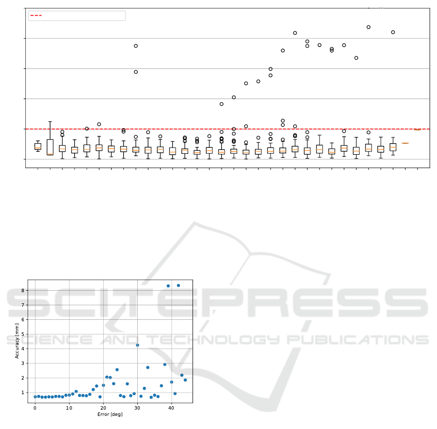
Robustness to Model Rotations

Generally speaking, the multi-view approach is not

invariant to rotation. The requirement of initial model

alignment stems from this matter of fact. Therefore,

we were interested in how the method performs with

increasing alignment error. With an alignment error

of less than 20 degrees, the method brings sufﬁciently

accurate predictions. With higher alignment errors,

especially above 30 degrees, the results should be vi-

sually checked and if needed, manually ﬁxed. This

correlation is depicted in Figure 8.

2.0

2.5

4.0

Acceptance value (mm)

100

SDR (%)

78.32

93.36

97.98

98.07

1 view

9 views

25 views

100 views

Figure 6: Success Detection Rates (SDRs) for Attention U-

Net, 2-channel input and the RANSAC consensus method.

Assuming the acceptable distance is 2 mm, setting the num-

ber of viewpoints higher than 25 does not bring any signiﬁ-

cant increase in performance.

5.3 Detection of Teeth Presence

The main focus of the experiments was to determine

whether the method’s self-evaluation can detect the

presence of landmarks (and therefore, teeth). In line

with previous studies in uncertainty measures, each

prediction’s peak value is considered one of the de-

cision factors. Networks were trained by regressing

heatmaps containing a Gaussian activation with the

amplitude of 1. The predictions should follow the

similar trend. There was no Gaussian in the ground

Robust Teeth Detection in 3D Dental Scans by Automated Multi-view Landmarking

L8D

L8M

L7D

L7M

L6D

L6M

L5D

L5M

L4D

L4M

L3D

L3M

L2D

L2M

L1D

L1M

R1M

R1D

R2M

R2D

R3M

R3D

R4M

R4D

R5M

R5D

R6M

R6D

R7M

R7D

R8M

R8D

Landmark

Distance from GT (mm)

Acceptable distance (2 mm)

Figure 7: Box plots of the radial error values of individual landmarks. These values were measured with following method

conﬁguration: Attention U-Net, two-channel input, 25 views, and RANSAC consensus method. Additionally, the class-

balanced loss was used for training. The landmark notation describes the type of landmark as follows: L stands for Left

dentition part and R for Right, values 1 - 8 describe tooth in the quadrant (1 for centran incisor and 8 for 3rd molars) and

letters M and D stand for mesial and distal landmark, respectively. Note that the outlier values in Right dentition part were

caused by one problematic case, where all teeth in right part were shifted by one and our method misclassiﬁed each tooth with

its adjacent tooth.

Figure 8: Correlation between error from required align-

ment and landmarking accuracy. As the 3D model is ob-

served from different angles, the method robustly estimates

landmarks even when the model is slightly rotated. Over-

all, the method becomes less stable with increasing error in

alignment, especially above 30 degrees.

truth image if a landmark was missing on the polyg-

onal model during training. This implies that the pre-

dictions should be either heatmaps with a peak value

close to 1 or heatmaps with all values close to 0.

By plotting an ROC curve, it was found that the

threshold value that brings off the best sensitivity and

speciﬁcity values is 0.375. Please note that this value

should be always cross-validated for each task. The

accuracy of the detection was 96.36%. After em-

pirical observations, there were situations where on

a tooth, one landmark was classiﬁed as missing and

the second one as present. This undesirable situa-

tion was eliminated by measuring the certainty in cou-

ples, averaging its conﬁdences. It leads to better re-

sults, even if the improvement is negligible, achiev-

ing an accuracy of 96.69%. Another promising ﬁnd-

ing comes from the RANSAC consensus method out-

put. The Multi-view Conﬁdence, measured as the

ratio between inliers and outliers, was again moni-

tored by an ROC curve. The threshold was set to

0.85 and combined with the analysis of heatmap max-

imum value. Superior results are seen for this combi-

nation, as 97.68% of landmarks are correctly classi-

ﬁed as missing or present.

Detecting Presence of 3rd Molars

A special category of detected teeth is 3rd molars. As

discussed in Section 3, those teeth are represented in

approximately 15% of the cases. The approach uti-

lized for detection of teeth presence suffers from this

imbalance, as the 3rd molars were always classiﬁed as

missing. This was due to the training, where, in most

cases, wisdom teeth were not present. To address this

problem, the loss was balanced in class-wise man-

ner (Cui et al., 2019). With this technique, 9 out of 12

wisdom teeth in the test set were correctly detected.

BIOIMAGING 2022 - 9th International Conference on Bioimaging

0.0

2.0 mm

4.0 mm

6.0 mm

8.0 mm

10.0+ m

Figure 9: Examples of automatically detected landmarks

with our method. Majority of predictions have the landmark

localization error less than 2 mm. Our method correctly de-

tects if a tooth is missing and does not produce predictions

of corresponding landmarks.

6 CONCLUSIONS

The present ﬁndings conﬁrm that the multi-view

approach combined with the RANSAC consensus

method brings promising results in the automation of

landmark detection. Evaluated on a dataset of real or-

thodontics dental casts with signiﬁcant diversity, the

method performs the best with Attention U-Net archi-

tecture and with two-channeled input of depth maps

and geometry renders. This method setup achieves

a landmarking accuracy of 0.75 ± 0.96 mm.

Importantly, we have also shown that the uncer-

tainty measures based on the analysis of the max-

imum values of regressed heatmap predictions in

combination with multi-view uncertainty yield con-

venient information in the process of landmark pres-

ence detection. Combining these uncertainty mea-

sures, our method correctly detects landmark pres-

ence in 97.68% of cases. This means that the method

is suitable to be applied to data where landmarks’

presence is not granted. In addition, the method meets

the needs of clinical applications, as the inference at

the user’s side takes seconds to be calculated, even on

less powerful CPUs.

Even though the accuracies are satisfying, the size

of the dataset could not cover every bit of a maloc-

clusion case and teeth shifting. Future research could

examine the method on a larger dataset of dentition

with even more complex cases. Furthermore, future

studies should focus on the improvements in the in-

variance of rotation. The association between the ro-

tation from the aligned position and the landmarking

accuracy was investigated in this work, and it is the

main shortcoming of the proposed method.

ACKNOWLEDGEMENTS

This work was supported by TESCAN 3DIM, s.r.o.,

which provided us with the dataset used in this work

as well as with its funding.

REFERENCES

Cui, Y., Jia, M., Lin, T.-Y., Song, Y., and Belongie, S.

(2019). Class-balanced loss based on effective num-

ber of samples.

Donner, R., Menze, B. H., Bischof, H., and Langs, G.

(2013). Global localization of 3d anatomical struc-

tures by pre-ﬁltered hough forests and discrete opti-

mization. Medical Image Analysis, 17(8):1304–1314.

Drevick

y, D. and Kodym, O. (2020). Evaluating deep learn-

ing uncertainty measures in cephalometric landmark

localization. In Proceedings of the 13th International

Joint Conference on Biomedical Engineering Systems

and Technologies - BIOIMAGING,, pages 213–220.

INSTICC, SciTePress.

Fischler, M. A. and Bolles, R. C. (1981). Random sample

consensus: A paradigm for model ﬁtting with appli-

cations to image analysis and automated cartography.

Commun. ACM, 24(6):381–395.

Lv, J., Shao, X., Xing, J., Cheng, C., and Zhou, X.

(2017). A deep regression architecture with two-stage

re-initialization for high performance facial landmark

detection. In 2017 IEEE Conference on Computer Vi-

sion and Pattern Recognition, CVPR 2017, Honolulu,

HI, USA, July 21-26, 2017, pages 3691–3700. IEEE

Computer Society.

Normando, D. (2015). Third molars: To extract or not to ex-

tract? Dental press journal of orthodontics, 20(4):17–

18.

Paulsen, R. R., Juhl, K. A., Haspang, T. M., Hansen, T. F.,

Ganz, M., and Einarsson, G. (2018). Multi-view con-

sensus CNN for 3d facial landmark placement. In

Jawahar, C. V., Li, H., Mori, G., and Schindler, K.,

editors, Computer Vision - ACCV 2018 - 14th Asian

Conference on Computer Vision, Perth, Australia, De-

cember 2-6, 2018, Revised Selected Papers, Part I,

Robust Teeth Detection in 3D Dental Scans by Automated Multi-view Landmarking

volume 11361 of Lecture Notes in Computer Science,

pages 706–719, Cham. Springer.

Payer, C., Stern, D., Bischof, H., and Urschler, M. (2016).

Regressing heatmaps for multiple landmark localiza-

tion using cnns. In Ourselin, S., Joskowicz, L.,

Sabuncu, M. R.,

Unal, G. B., and Wells, W., editors,

Medical Image Computing and Computer-Assisted In-

tervention - MICCAI 2016 - 19th International Con-

ference, Athens, Greece, October 17-21, 2016, Pro-

ceedings, Part II, volume 9901 of Lecture Notes in

Computer Science, pages 230–238. Springer.

Pﬁster, T., Charles, J., and Zisserman, A. (2015). Flowing

convnets for human pose estimation in videos. In 2015

IEEE International Conference on Computer Vision,

ICCV 2015, Santiago, Chile, December 7-13, 2015,

pages 1913–1921. IEEE Computer Society.

Qi, C. R., Su, H., Mo, K., and Guibas, L. J. (2017). Pointnet:

Deep learning on point sets for 3d classiﬁcation and

segmentation.

Su, H., Maji, S., Kalogerakis, E., and Learned-Miller, E. G.

(2015). Multi-view convolutional neural networks for

3d shape recognition. In 2015 IEEE International

Conference on Computer Vision, ICCV 2015, Santi-

ago, Chile, December 7-13, 2015, pages 945–953.

IEEE Computer Society.

Sun, D., Pei, Y., Li, P., Song, G., Guo, Y., Zha, H., and Xu,

T. (2020). Automatic tooth segmentation and dense

correspondence of 3d dental model. In MICCAI.

Sun, Y., Wang, X., and Tang, X. (2013). Deep convolutional

network cascade for facial point detection. In 2013

IEEE Conference on Computer Vision and Pattern

Recognition, Portland, OR, USA, June 23-28, 2013,

pages 3476–3483. IEEE Computer Society.

Wu, T.-H., Lian, C., Lee, S., Pastewait, M., Piers, C., Liu, J.,

Wang, F., Wang, L., Jackson, C., Chao, W.-L., Shen,

D., and Ko, C.-C. (2021). Two-stage mesh deep learn-

ing for automated tooth segmentation and landmark

localization on 3d intraoral scans.

BIOIMAGING 2022 - 9th International Conference on Bioimaging