
U-Net based Semantic Segmentation of Kidney and Kidney Tumours of
CT Images
Benjamin Bracke and Klaus Brinker
Hamm-Lippstadt University of Applied Sciences, Marker Allee 76-78, 59063 Hamm, Germany
Keywords:
Medical Image Segmentation, Semantic Segmentation, Kidney Tumours Segmentation, U-Net, Deep Learn-
ing, Transfer Learning, Hyperparameter Optimization.
Abstract:
Semantic segmentation of kidney tumours in medical image data is an important step for diagnosis as well as
in planning and monitoring of treatments. Morphological heterogeneity of kidneys and tumours in medical
image data is a major challenge for automatic segmentation methods, therefore segmentations are typically
performed manually by radiologists. In this paper, we use a state-of-the-art segmentation method based on the
deep learning U-Net architecture to propose a segmentation algorithm for automatic semantic segmentation
of kidneys and kidney tumours of 2D CT images. Therefore, we particularly focus on transfer learning of U-
Net architectures and provide an experimental evaluation of different hyperparameters for data augmentation,
various loss functions, U-Net encoders with varying complexity as well as different transfer learning strategies
to increase the segmentation accuracy. We have used the results of the evaluation to fix the hyperparameters
of our final segmentation algorithm, which has achieved a high segmentation accuracy for kidney pixels and a
lower segmentation accuracy for tumor pixels.
1 INTRODUCTION
In 2020, more than 430,000 kidney tumours were
diagnosed worldwide, nearly 40% resulted in death
(Sung et al., 2021). Medical imaging techniques such
as computed tomography (CT) play a central role in
the diagnosis of kidney tumours as well as in plan-
ning and monitoring of treatment steps. Currently,
analysing medical image data for precise localiza-
tion and segmentation of kidney- and kidney tumours
tissue is a manual and time-consuming process per-
formed by radiologists (S. Kevin Zhou, 2020). There-
fore, image segmentation techniques that can recog-
nize related features in medical image data and assign
a specific class (e.g. background, kidney or tumour)
to each pixel could support the work of radiologists by
automatically pre-segmenting the image data. How-
ever, the morphological heterogeneity of medical im-
age data has been a major challenge for automatic im-
age segmentation methods for a long time.
In recent years, major progress has been made
in machine learning, which has also led to new and
more powerful image segmentation methods based
on artificial neural networks (Litjens et al., 2017),
such as the deep learning U-Net architecture pre-
sented by Ronneberger et al. U-Nets are encoder-
decoder architectures based on fully Convolutional-
Neural-Networks (FCN) that combine a contractive
path for learnable feature extraction and an expansive
path with skip connections between encoder and de-
coder for learnable upscaling of the extracted features
(Ronneberger et al., 2015). In the past, U-Nets have
been successfully used for segmentation of medical
image data and in some applications have even been
able to achieve better segmentation accuracy than ra-
diologists (Litjens et al., 2017).
This paper picks up on the success of U-Nets and
aims to develop a segmentation algorithm for seman-
tic segmentation of kidney tissue and kidney tumours
tissue from 2D CT image data. To achieve this objec-
tive, we will focus on transfer learning of existing and
pre-trained U-Net architectures as well as on the opti-
mization of its so-called hyperparameters, which are
not trained automatically but have to be set manually.
Therefore, we investigate in detail how different hy-
perparameters related to the data augmentation, loss
function, U-Net encoders and transfer learning affect
the segmentation accuracy.
In the following, we first introduce the considered
dataset as well as different methods considered in the
optimization of the U-Net hyperparameters. Then, the
effects of the introduced methods on the segmentation
accuracy are evaluated and discussed using empirical
experiments, while the best methods will be included
in our proposed segmentation algorithm. Finally, a
conclusion is given.
Bracke, B. and Brinker, K.
U-Net based Semantic Segmentation of Kidney and Kidney Tumours of CT Images.
DOI: 10.5220/0010770900003123
In Proceedings of the 15th International Joint Conference on Biomedical Engineering Systems and Technologies (BIOSTEC 2022) - Volume 2: BIOIMAGING, pages 93-102
ISBN: 978-989-758-552-4; ISSN: 2184-4305
Copyright
c
2022 by SCITEPRESS – Science and Technology Publications, Lda. All rights reserved
93

2 MATERIAL AND METHODS
In this section, we will start with a description of the
considered dataset and explain necessary adjustments
and pre-processing steps. Afterwards, we present dif-
ferent methods considered in the optimization of the
U-Net hyperparameters, which concern data augmen-
tation, a suitable loss function for segmentation tasks
and transfer learning of a U-Net architecture.
2.1 KiTS19 Dataset
The data used in this paper is derived from the ”Kid-
ney Tumor Segmentation 2019 (KiTS19)” dataset
(Heller et al., 2019), which was released as a train-
ing dataset as part of a Grand-Challenge
1
under the
creative commons license CC BY-NC-SA on March
15, 2019. It includes three-dimensional computed to-
mography images (CT volumes) of 210 patients who
underwent nephrectomy at the University of Min-
nesota Medical Center. This dataset provides three-
dimensional ground truth segmentations which assign
the voxels of a CT volume to either the ”kidney”, ”tu-
mour” or ”background” class, depending on the rep-
resented tissues. The CT volumes and segmentations
have a spatial resolution of 512x512 voxels along the
x- and y-dimensions, while the number of acquisition
slices (z-dimension) varies between patients.
2.2 Pre-processing
We conducted some adjustments and pre-processing
on the KiTS19 dataset, which are briefly explained
in the following. Since this paper focuses on two-
dimensional semantic segmentation, individual trans-
verse CT images were extracted from the acquisition
slices of each patient’s three-dimensional CT volume.
As a result, a total of 45,424 individual CT images
were extracted from all 210 CT volumes, of which
the majority (≈64%) only contained the background
class. About 23.4% of the images contained the
classes background and kidney while approx. 11.5%
contained all classes background, kidney and tumour.
About 1.1% only contained the classes background
and tumour. The high number of CT images contain-
ing only the background class does not provide further
information about kidneys or tumours to the segmen-
tation algorithm and could instead negatively impact
training success and increase training run times. Con-
sequently, most of these CT images were removed
and only 1% (at least one image) per CT volume were
retained. As a result of this filtering, only around 37%
(16,795) of the extracted CT images remain. As the
1
https://kits19.grand-challenge.org/
number of acquisition slices of the patient CT vol-
umes varies, the number of extractable CT images
differs per patient. As a result, patients with many CT
images would have a greater influence in training and
in evaluation than patients with fewer CT images. To
balance the influence of patients and avoid this bias,
each CT image was weighted by a specific parameter.
This parameter is equivalent to the inverse of the ex-
tracted and filtered number of CT images of a patient.
During preprocessing, the intensity windows of the
CT images were first clipped to [-125,225] Hounsfield
units to achieve high contrast for the soft tissue of the
abdomen and then normalized to the interval [0,1].
Also, the resolution of the CT images were reduced
from 512x512 pixels to 256x256 pixels to decrease
the processing time in the training process. All CT
images were divided into training, validation, and test
data on the patient level. From a total of 210 patients,
74 patients (≈35%) were designated as test dataset,
116 patients (≈55%) as training dataset and 20 pa-
tients (≈10%) as validation dataset. Altogether, the
test dataset provides a total of 5,494 CT images, the
training dataset a total of 9,590 CT images, and the
validation dataset a total of 1,711 CT images.
2.3 Data Augmentation
A major limiting factor when training artificial neu-
ral networks is the amount of available training data.
The KiTS19 training dataset provides only a limited
number of training data and consequently only low
variability, which may lead to problems in training,
such as overfitting and an overall poor generaliza-
tion performance. Access to further training data
with ground truth segmentations matching the topic
of this paper is limited, so data augmentation tech-
niques are used to artificially increase the variability
of the training data by modifying them using various
transformations. For this purpose, a data augmenta-
tion pipeline was developed, which combines spatial
transformation methods like flipping, rotation, elastic
transformation, grid distortion, crop or pad as well as
intensity transformations like brightness-, contrast-,
gamma adjustments, blurring, adding noise or com-
pression artefacts. Data augmentation is performed
dynamically for each CT image during the training
process. Which transformation methods are used for
data augmentation is determined randomly per image
with a probability of 50% per transformation method.
To prevent including only augmented images, the pro-
portion of data augmentation can be specified by a
hyperparameter. We will empirically evaluate this hy-
perparameter to determine the best proportion of data
augmentation in terms of segmentation accuracy.
BIOIMAGING 2022 - 9th International Conference on Bioimaging
94
2.4 Loss Functions
Another important hyperparameter in training of ar-
tificial neural networks is the loss function, which
quantifies the deviation between the networks predic-
tion and the ground truth and should be minimized
during the training process. A common problem in
medical image data segmentation is the handling of
class imbalances. The proportion of pixels that a kid-
ney or tumour represents in a CT image is usually
very small, resulting in a skewed distribution in favour
of background pixels. Under these circumstances, a
careful selection of a loss function that takes the un-
balanced pixel distribution of each class into account
is crucial. Therefore, we consider different loss func-
tions and empirically evaluate which loss function is
best suited in terms of segmentation accuracy for the
purpose of this paper.
2.4.1 Cross Entropy
When cross entropy (CE) is used as a loss function
for segmentation tasks, a loss is determined between
predictions (p) and ground truth (g) for each pixel
(i) and then averaged over all pixels (N). The cross
entropy does not consider the class imbalance prob-
lem mentioned earlier. Therefore, we also consider
a weighted cross entropy (WCE), which weights the
pixel losses of each class (c) differently. The weight-
ing parameters (w
c
) of each class are calculated using
the ”Median-Frequency-Balancing” (Eigen and Fer-
gus, 2014).
CE = −
1
N
N
∑
i=1
C
∑
c=1
g
i,c
· log(p
i,c
) (1)
WCE = −
1
N
N
∑
i=1
C
∑
c=1
w
c
· g
i,c
· log(p
i,c
) (2)
2.4.2 Dice Loss
We also investigate the dice loss (Sudre et al.,
2017) function based on the Sørensen-Dice coeffi-
cient (DSC), which characterises the overlap between
the prediction (p) and ground truth (g) and is there-
fore robust to different pixel proportions of the classes
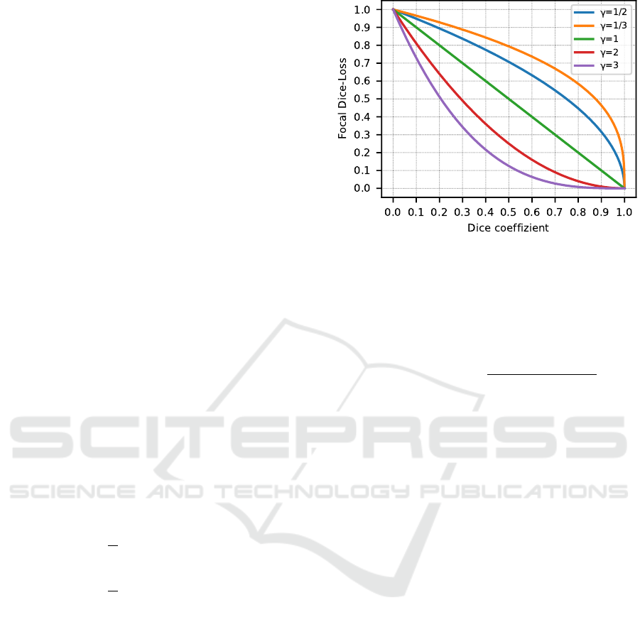
(c). Furthermore, we want to consider focusing of the
dice loss similar to the Focal-Tversky loss (Abraham
and Khan, 2018). Focusing is done by a γ-parameter,
which exponentiates the dice loss for each class re-
spectively. The effects of focusing are shown in Fig-
ure 1. Essentially, with a γ-value < 1, the loss is
higher for images with dice coefficients > 0.5, which
allows focusing on images that are easy-to-segment
(Abraham and Khan, 2018). The opposite case is true
Figure 1: Focusing effects of the Focal-Dice loss compared
to the dice coefficient. A focusing of γ = 1 corresponds to
the unfocused Dice loss.
for a γ-value > 1 and allows focusing on harder-to-
segment images. Both focusing cases will be empiri-
cally evaluated in this paper.
DSC
c
=
2
∑
N
i=1
p
i,c
g
i,c
∑
N
i=1
p
i,c
+
∑
N
i=1
g
i,c
(3)
Dice Loss =
C
∑
c=1
(1 − DSC
c
) (4)
Focal-Dice Loss =
C
∑
c=1
(1 − DSC
c
)
γ
(5)
2.5 Transfer-learning
Due to the limited amount of training data, this pa-
per focuses on transfer learning and uses pre-trained
Convolutional-Neural-Networks as a base model for
the U-Net encoder. Which base model is best suited
as a U-Net encoder will be evaluated empirically. For
this purpose, we analyse how different variants of the
ResNet architecture (He et al., 2015) like ResNet18,
ResNet34, ResNet50 and ResNet101, which differ
mainly in complexity due to a different number of
convolutional layers, affect the segmentation accu-
racy. These pre-trained ResNet models have already
learned a general feature extraction representation
from the large ImageNet dataset, so only an optimiza-
tion of the feature extraction with respect to the ap-
plication field of this paper is required by re-training
some layers. How far the optimization by re-training
certain layers affects the segmentation accuracy will
also be evaluated empirically. The U-Net decoder,
which is designed to expand symmetrically to the
stages of the ResNet architecture, is initialized ran-
domly and must therefore be retrained each time.
U-Net based Semantic Segmentation of Kidney and Kidney Tumours of CT Images
95

2.6 Implementation
The segmentation algorithm with the previously de-
scribed methods was implemented in Python 3.9.4,
with the help of the libraries Tensorflow 2.4.1 and
Numpy 1.20.1. The used U-Net architectures derive
from the library Segmentation Models 1.0.1
2
and data
augmentation was done with the libraries Albumenta-
tions 0.5.2 and OpenCV 4.5.2. The experiments for
evaluation were performed on an Ubuntu 18.04 server
with four Nvidia RTX 2080TI graphics cards, 128GB
memory and two Intel Xeon Silver 4110 CPUs.
3 EVALUATION
In this section, we evaluate how the different consid-
ered methods for the U-Net architecture and hyper-
parameters for training affect the segmentation accu-
racy. First, we describe the performed evaluation ap-
proach. Then, the evaluation results of the considered
methods and the results of the final segmentation al-
gorithm are presented.
3.1 Approach
To determine how the different considered methods
for the U-Net architecture and training hyperparame-
ters affect the segmentation accuracy, several empir-
ical experiments are conducted. Testing all possible
combinations of the hyperparameters would be com-
putationally too extensive, so instead we followed a
stepwise approach.
For this purpose, all hyperparameters were first set
manually as shown in Table 1. Starting from these
initial hyperparameters, only one hyperparameter was
evaluated at a time in sequential experiments. De-
pendencies between hyperparameters require careful
consideration of the experimental sequence. There-
fore, we first evaluated the hyperparameter of the data
augmentation proportion to minimize early overfitting
effects during the experiments, especially when train-
ing more complex U-Net encoders. The hyperparam-
eter for the data augmentation proportion was then in-
cluded in the second experiment, in which we evalu-
ate the optimal loss function. Following the same ap-
proach, we decided to determine the optimal U-Net
encoder and the hyperparameters for transfer learn-
ing in the last two experiments. All evaluated hyper-
parameters were then combined to train a final seg-
mentation algorithm. During the experiments, differ-
ent U-Net models were trained with a learning rate of
2
https://github.com/qubvel/segmentation models
Table 1: Initialization hyperparameters of the experiments.
Data Aug.
Proportion
Loss
Function
U-Net
Encoder
Re-Trained
Layers
0% Dice Loss ResNet34 from Stage 3
10
−5
, a batch size of 24 CT images and a relatively
short training period of 50 epochs to further reduce
the computational cost, Afterwards, the segmentation
accuracy for each model was evaluated using super-
vised pixel-based evaluation metrics over the entire
validation dataset. We mainly focused on the eval-
uation metrics dice coefficient, recall and precision,
that consider the classification cases of true positive
(TP), false positive (FP), and false negative (FN) of
each pixel in the segmented image with respect to the
ground truth image (Taha and Hanbury, 2015). To
minimize variations that may occur due to random in-
fluences in the training process, each experiment was
repeated four times, and the mean and standard devi-
ation of the metrics were used for evaluation.
Dice coefficient =
2T P
2T P + FP + FN
(6)
Recall =
T P
T P + FN
(7)
Precision =
T P
T P + FP
(8)
3.2 Hyperparameter Optimization
In the following, the evaluation results of each hyper-
parameter experiment are presented and it is briefly
mentioned which hyperparameter is used for the fol-
lowing experiment. A more detailed discussion is
given in section 4.
3.2.1 Impact of Data Augmentation Proportion
The aim of the first experiment was to determine
how different data augmentation proportions affect
the segmentation accuracy. For this purpose, sev-
eral U-Net models were trained using different data
augmentation proportions p∈[0%, 25%, 50%, 75%,
80%, 90%, 100%]. The data augmentation proportion
p=0% is equivalent to no data augmentation.
Considering the results of the evaluation metrics,
dice coefficient in Figure 2 and recall in Table 2, a
clear trend can be seen. With increasing data augmen-
tation proportion from p=0% to p=75%, an improve-
ment in segmentation accuracy can be observed. This
improvement is particularly noticeable for the tumour
class, where an approximately 13.5% higher dice co-
efficient and approximately 25.2% higher recall is
achieved. In contrast, only minor fluctuations are ob-
served for the kidney and background classes, which
BIOIMAGING 2022 - 9th International Conference on Bioimaging
96
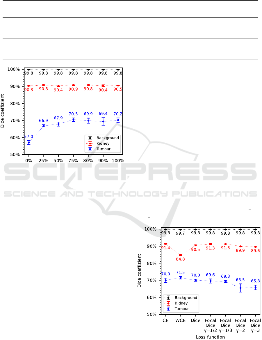
Table 2: Evaluation results of recall and precision for the analyzed data augmentation proportions.
Class
Data Augmentation Proportion
0% 25% 50% 75% 80% 90% 100%
Recall
Background 99.9% ±0.0 99.9% ±0.0 99.9% ±0.1 99.9% ±0.1 99.9% ±0.0 99.9% ±0.0 99.9% ±0.0
Kidney 87.3% ±0.4 87.7% ±0.5 87.1% ±1.0 88.1% ±0.8 88.0% ±0.6 87.2% ±1.1 87.2% ±0.4
Tumour 51.7% ±2.3 69.8% ±3.0 75.6% ±1.0 76.9% ±2.6 75.2% ±2.4 74.8% ±1.8 77.0% ±1.7
Precision
Background 99.7% ±0.0 99.8% ±0.0 99.8% ±0.0 99.8% ±0.0 99.8% ±0.0 99.8% ±0.0 99.8% ±0.0
Kidney 93.5% ±0.3 94.1% ±0.4 93.9% ±0.4 94.0% ±0.2 93.7% ±0.3 93.9% ±0.3 94.2% ±0.2
Tumour 63.7% ±0.9 64.3% ±2.3 61.7% ±1.9 65.4% ±3.1 65.3% ±0.9 64.8% ±3.3 64.5% ±2.1
Data Augmentation Proportion
Figure 2: Evaluation results of the dice coefficient for the
analyzed data augmentation proportions.
show no clear improvement in segmentation accu-
racy. At even higher data augmentation proportions
of p>75%, no further improvement in segmentation
accuracy is noticeable for the tumour class. Rather, a
saturation of the dice coefficient at around 70% and
for recall of around 75% to 77% is noticeable. There
are only minor fluctuations in the evaluation results of
the precision metric with partly high standard devia-
tions, which do not indicate a clear trend.
According to these results, a data augmentation
proportion of p=75% is selected as a hyperparameter
for the following experiments as well as for the final
segmentation algorithm.
3.2.2 Impact of Loss Function
The aim of the second experiment was to determine
the effect of different loss functions on the segmenta-
tion accuracy. For this purpose, various U-Net models
were trained using different loss functions in the train-
ing process. The influence of cross entropy versus
weighted cross entropy was evaluated with weighting
parameters of 0.02 for the background class, 1.0 for
the kidney class and 1.5 for the tumour class. We
also evaluated the influence of the dice loss on the
segmentation accuracy and whether focusing the dice
loss with varying γ-values of g∈[
1
2
,
1
3
, 2, 3] is useful.
The evaluation results of this experiment with re-
spect to the dice coefficient are shown in Figure 3
as well as the results for recall and precision in Ta-
ble 3. Comparing the evaluation results of the loss
function cross entropy with those of the weighted
cross entropy, the weighted cross entropy achieves
higher recall results of about 3.9% for the kidney
class and about 7.5% for the tumour class. In con-
trast, the other evaluation metrics show a significantly
worse segmentation accuracy of the weighted cross
entropy compared to the cross entropy. This is partic-
ularly noticeable in the dice coefficient, which is ap-
proximately 6.6% lower for the kidney class, and for
the precision metric, which is approximately 15.8%
lower. For the tumour class, there is only a slight im-
provement of about 1.5% in the dice coefficient with
the weighted cross entropy, but also a significantly
lower precision of about 3.7%. Comparing the evalu-
ation results of the dice loss with the focused variants
of the dice loss to easy-to-segment images (γ =
1
2
and
γ =
1
3
), only slight differences in segmentation accu-
Figure 3: Evaluation results of the dice coefficient for the
analyzed loss functions.
U-Net based Semantic Segmentation of Kidney and Kidney Tumours of CT Images
97
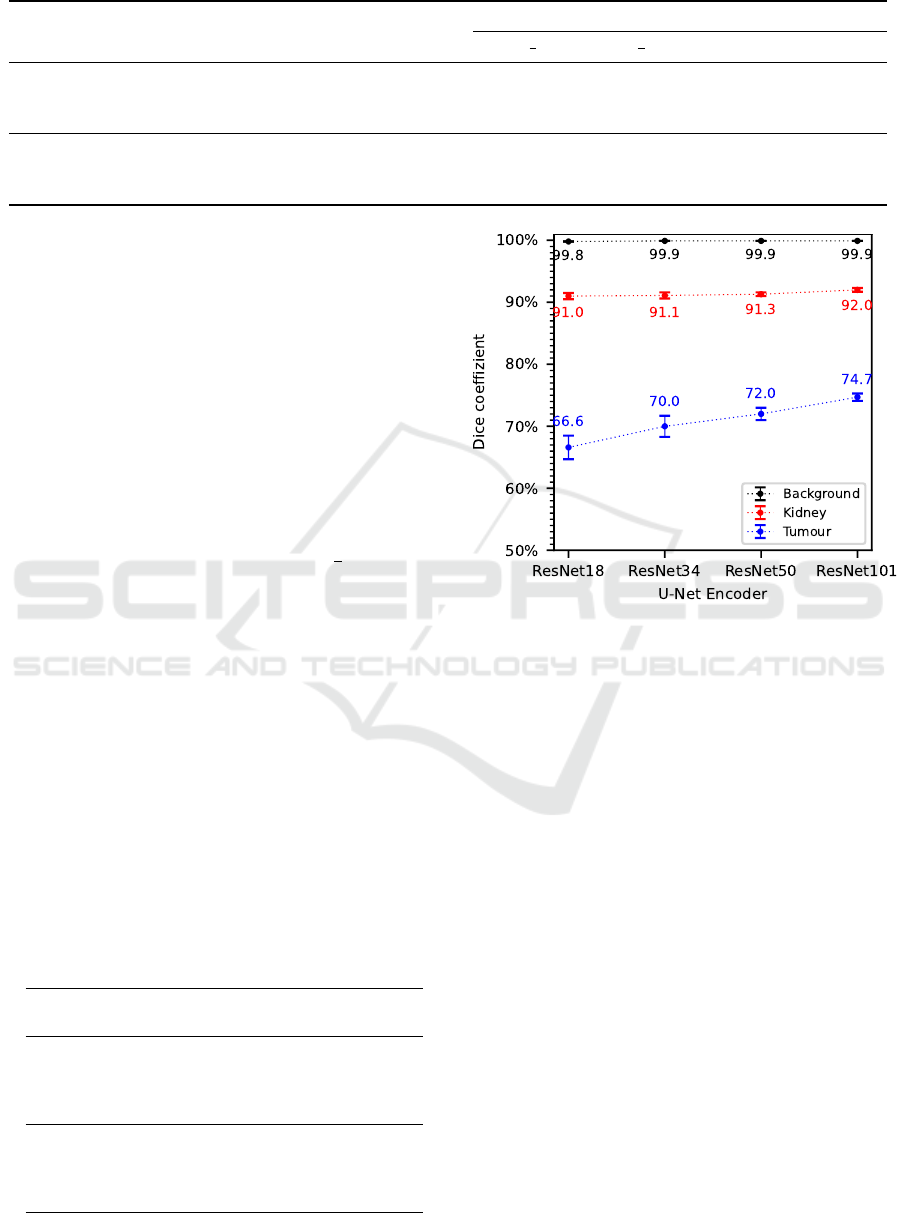
Table 3: Evaluation results of recall and precision for the analyzed loss functions.
Class
CE
Loss
WCE
Loss
Dice
Loss
Focal-Dice Loss
γ =
1
2
γ =
1
3
γ = 2 γ = 3
Recall
Background 99.9% ±0.0 99.4% ±0.0 99.9% ±0.0 99.9% ±0.0 99.9% ±0.0 99.8% ±0.0 99.8% ±0.1
Kidney 89.0% ±0.3 92.9% ±0.7 87.4% ±1.0 88.4% ±0.7 88.4% ±0.4 87.3% ±0.4 86.6% ±0.2
Tumour 69.4% ±0.8 76.9% ±1.5 77.9% ±1.0 73.4% ±0.8 73.7% ±2.1 66.5% ±3.2 67.0% ±2.0
Precision
Background 99.8% ±0.0 99.9% ±0.0 99.8% ±0.0 99.8% ±0.0 99.8% ±0.0 99.7% ±0.0 99.7% ±0.0
Kidney 93.8% ±0.1 78.0% ±0.5 93.9% ±0.5 94.2% ±0.1 94.4% ±0.3 92.6% ±0.1 92.7% ±0.3
Tumour 70.5% ±1.8 66.8% ±0.7 63.6% ±1.3 66.1% ±2.4 65.4% ±1.4 64.6% ±1.7 64.6% ±1.5
racy can be observed. These are mainly evident in a
slightly better dice coefficient, recall and precision of
the kidney class regarding the focused loss variants,
but also in a slightly worse dice coefficient and recall
of the tumour class. In general, recall and precision
of the tumour class are more balanced for the focused
loss variants than for the normal dice loss. Focusing
on harder-to-segment images (γ = 2 and γ = 3) results
in a significantly worse segmentation accuracy com-
pared to the normal dice loss, as evidenced by approx-
imately 4.3% lower dice coefficient and the approxi-
mately 10% lower recall of the tumour class.
Considering the more balanced recall and preci-
sion results and the high dice coefficient, the focused
dice loss on easy-to-segment images (γ =
1
2
) is chosen
as a hyperparameter for the following experiments as
well as for the final segmentation algorithm.
3.2.3 Impact of U-Net Encoder
The aim of the third experiment was to determine the
effects of different U-Net encoders of varying com-
plexity in terms of segmentation accuracy. Therefore,
various U-Net models were trained using four differ-
ent Convolutional-Neural-Networks of the ResNet ar-
chitecture as a basis for the U-Net encoder, including
the ResNet18, ResNet34, ResNet50, and ResNet101.
Considering the results of the evaluation metrics
dice coefficient in Figures 4 as well as recall and
precision in Table 4, a trend is noticeable that with
Table 4: Evaluation results of recall and precision for the
analysed U-Net encoders.
U-Net
Encoder
Background Kidney Tumour
Recall
ResNet18 99.9% ±0.0 87.7% ±1.1 66.4% ±2.2
ResNet34 99.9% ±0.0 88.1% ±1.0 75.5% ±1.8
ResNet50 99.9% ±0.0 88.8% ±0.7 74.4% ±3.4
ResNet101 99.9% ±0.0 89.6% ±0.7 79.9% ±1.6
Precision
ResNet18 99.8% ±0.1 94.4% ±0.4 67.0% ±3.4
ResNet34 99.8% ±0.0 94.5% ±0.2 65.3% ±2.6
ResNet50 99.8% ±0.0 93.9% ±0.3 69.9% ±2.0
ResNet101 99.8% ±0.0 94.6% ±0.3 70.9% ±1.8
Figure 4: Evaluation results of the dice coefficient for the
analysed U-Net encoders.
increasing complexity of the U-Net encoder an im-
provement in segmentation accuracy can be observed.
This improvement in segmentation accuracy is again
particularly noticeable in the tumour class, where the
dice coefficient increased by an average of 2.7% with
increasing complexity of the U-Net encoder. Recall
improves by about 12.6% for the ResNet101 com-
pared to the ResNet18, whereas precision increases
by just 2.9%. For the kidney class, there is only a
slight improvement in segmentation accuracy with in-
creasing complexity of the U-Net encoder, while no
significant changes occur for the background class.
According to these results, a U-Net encoder based
on the most complex ResNet101 architecture is cho-
sen as a basis for the following experiments as well as
for the final segmentation algorithm.
3.2.4 Impact of Transfer-learning
The aim of the fourth experiment was to determine
how the optimization of the pre-trained U-Net en-
coder (ResNet101) by re-training different numbers
of layers affects the segmentation accuracy. To evalu-
ate this, various U-Net models were trained in which
BIOIMAGING 2022 - 9th International Conference on Bioimaging
98
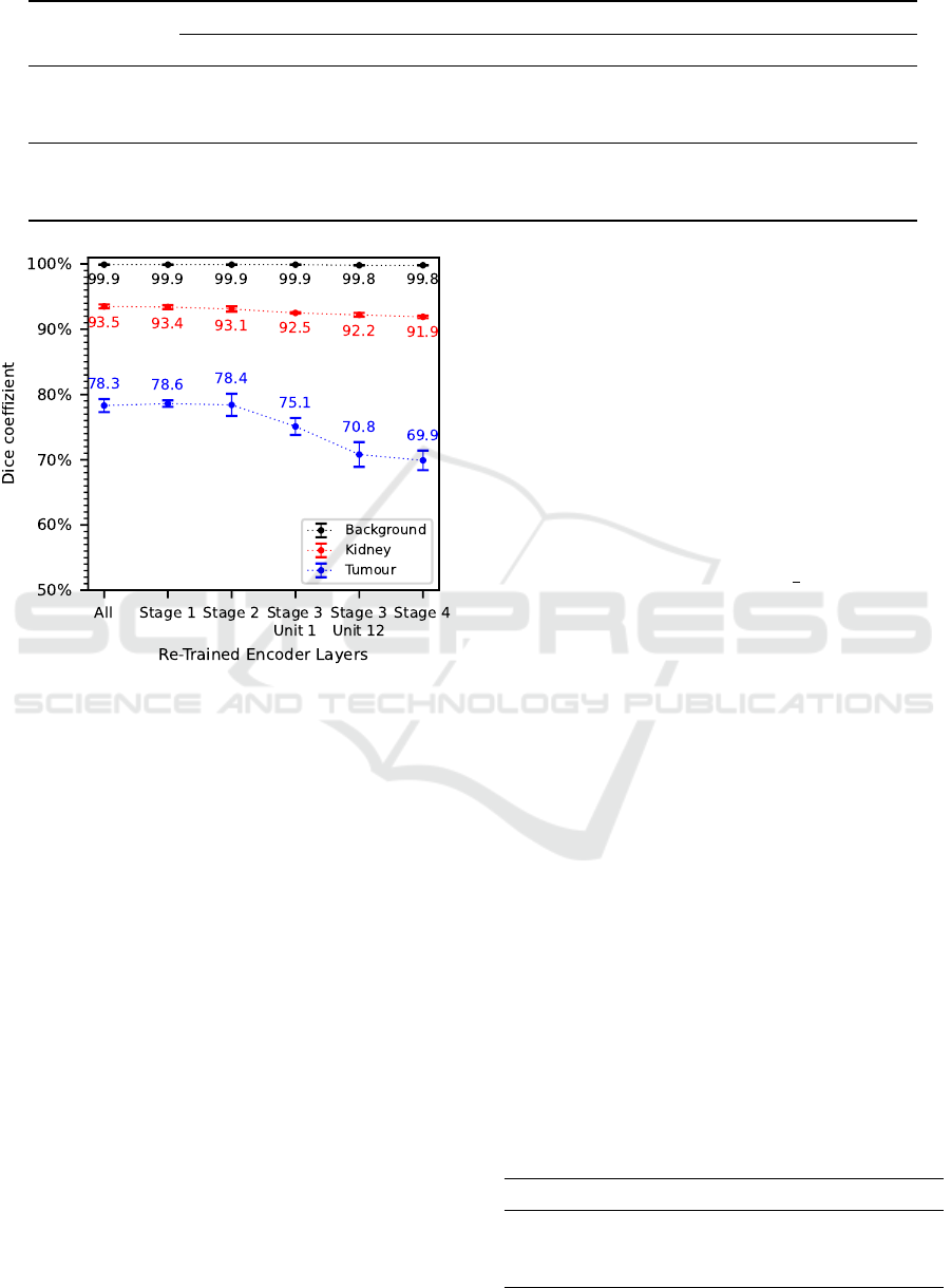
Table 5: Evaluation results of recall and precision for different numbers of re-trained encoder layers.
Class
Re-Trained Encoder Layers from:
All Stage 1 Stage 2 Stage 3 Unit 1 Stage 3 Unit 12 Stage 4
Recall
Background 99.9% ±0.0 99.9% ±0.0 99.9% ±0.0 99.9% ±0.0 99.9% ±0.1 99.9% ±0.0
Kidney 91.5% ±0.8 91.4% ±0.5 91.3% ±1.0 90.0% ±0.2 90.0% ±0.2 89.5% ±0.5
Tumour 80.0% ±2.4 82.4% ±1.4 81.3% ±0.8 78.3% ±4.1 79.8% ±0.2 71.5% ±0.6
Precision
Background 99.9% ±0.0 99.9% ±0.0 99.9% ±0.0 99.8% ±0.1 99.9% ±0.0 99.8% ±0.0
Kidney 95.4% ±0.2 95.5% ±0.1 95.0% ±0.3 95.0% ±0.2 94.6% ±0.4 94.4% ±0.2
Tumour 76.8% ±2.1 75.3% ±0.2 75.8% ±3.3 72.4% ±1.5 63.6% ±3.1 68.4% ±3.3
Figure 5: Evaluation results of dice coefficient for different
numbers of re-trained encoder layers.
the neuron weights of several encoder layers were
frozen to prevent them from being adjusted during the
training process. First, a model is trained in which
all encoder layers are re-trained and then models in
which the encoder layers starting from ResNet-Stage
1, Stage 2, Stage 3 Unit 1 (Unit = Residual Block),
Stage 3 Unit 12 and Stage 4 are re-trained.
Considering the results of the evaluation metrics
dice coefficient in Figure 5 as well as recall and preci-
sion in Table 5, a clear trend is noticeable. In general,
the segmentation accuracy decreases with decreasing
number of re-trained encoder layers. Larger differ-
ences occur in dice coefficient and precision when
only the encoder layers from Stage 3 and above are
re-trained, whereas similar results are obtained when
all encoder layers or the encoder layers starting from
Stage 1 or 2 are re-trained. This trend is especially no-
ticeable in the tumour class, where an approximately
8.4% higher dice coefficient and precision as well
as an approximately 8.5% higher recall are achieved
when all encoder layers are re-trained compared to re-
training only the encoder layers from Stage 4. For the
kidney class, this decreasing trend is only noticeable
to a minor degree while for the background class it is
hardly noticeable at all.
As a result, all encoder layers are re-trained for
transfer learning of the final segmentation algorithm.
3.3 Final Segmentation Algorithm
The aim of the previously performed experiments was
to determine the optimal hyperparameters for the fi-
nal segmentation algorithm as well as the final train-
ing process. As a result, of our evaluation the final
training should use a data augmentation proportion of
p=75% and a more focused variant of the dice loss
on easy-to-segment images (γ =
1
2
). Also, we de-
termined that the best transfer learning basis for the
final segmentation algorithm should be a pre-trained
ResNet101 encoder, where all encoder layers should
be re-trained. The same hyperparameters for learning
rate and batch size were used in the final training pro-
cess as in the previous experiments. Due to a lower
computational cost for the evaluation, the number of
training epochs of the experiments was limited to 50,
which was negligible for the final training. Therefore,
the number of training epochs was extended to 150 to
benefit from a longer training period. For the reasons
explained in section 3.1, the final training process was
also repeated four times and segmentation accuracy
was evaluated using the averaged results of the evalu-
ation metrics over the entire test dataset.
The evaluation result of the final segmentation al-
gorithm is presented in Table 6 as well as in the con-
fusion matrix in Figure 6. In addition, Figure 7 illus-
trates examples of the segmentation result. As can
be seen in the clear diagonal of the confusion ma-
trix, most of the pixels of the test dataset were seg-
Table 6: Evaluation results of dice coefficient, recall and
precision for the final segmentation algorithm.
Metric Background Kidney Tumour
Dice coeff.
99.9% ±0.0 94.7% ±0.1 84.5% ±0.4
Recall 99.9% ±0.0 94.8% ±0.1 81.2% ±1.0
Precision 99.9% ±0.0 94.6% ±0.3 88.1% ±0.4
U-Net based Semantic Segmentation of Kidney and Kidney Tumours of CT Images
99
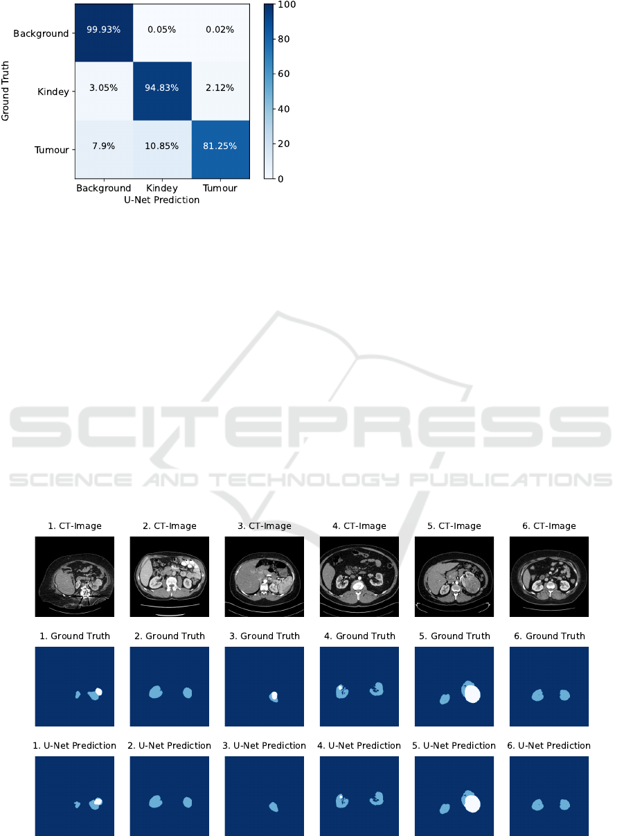
Figure 6: Normalized confusion matrix visualizing the seg-
mentation accuracy of the final segmentation algorithm.
mented with high accuracy. However, significant dif-
ferences in segmentation accuracy can be observed
for the individual classes. With approximately 99.9%
for the dice coefficient, recall and precision, the fi-
nal segmentation algorithm achieved a very high seg-
mentation accuracy for background pixels. A lower
segmentation accuracy of about 94% for the dice co-
efficient, recall and precision was achieved for kid-
ney pixels. According to the confusion matrix, only
3.05% were incorrectly predicted as background pix-
els and 2.12% as tumour pixels. A significantly lower
segmentation accuracy was achieved for tumour pix-
els, resulting in only about 81.25% correctly pre-
dicted tumour pixels. In contrast, the precision of
tumour pixels is significantly higher with approxi-
mately 88.1%. According to the confusion matrix,
the final segmentation algorithm misclassified a large
proportion of tumour pixels of about 10.85% as kid-
ney pixels and about 7.9% as background pixels.
4 DISCUSSION
The purpose of this paper was to develop a U-Net-
based segmentation algorithm for automated semantic
segmentation of kidneys and kidney tumours from 2D
medical CT images. Therefore, we mainly focused on
transfer learning and determined the optimal hyperpa-
rameters for the U-Net based segmentation algorithm
in various sequential experiments to increase the over-
all segmentation accuracy.
4.1 Data Augmentation Proportion
First, we experimented with the hyperparameter for a
different data augmentation proportion to investigate
the influence on the segmentation accuracy. The re-
sults have shown that with increasing data augmen-
tation proportion, a significant improvement in seg-
mentation accuracy was achieved, especially for the
tumour class. This trend was noticeable up to a data
augmentation proportion of p=75%, after which no
further improvements in segmentation accuracy oc-
curred. The obtained results confirm the previously
made assumption that the considered training dataset
provides only a low variability, which can be signif-
icantly increased by data augmentation and is there-
fore highly recommended. Data augmentation pro-
Figure 7: Examples of the segmentation results of the final segmentation algorithm. Dark blue regions represent the back-
ground class, light blue regions the kidney class and white regions the tumor class.
BIOIMAGING 2022 - 9th International Conference on Bioimaging
100

portions of p>75% may have resulted in an excessive
variability of the training data, preventing further im-
provements in segmentation accuracy in the limited
number of training epochs of this experiment. Per-
haps increasing the number of training epochs would
produce larger differences. As a consequence of these
results, we decided to select a data augmentation pro-
portion of p=75% as hyperparameter for the following
experiments and for the final segmentation algorithm.
4.2 Loss Function
Second, we considered different loss functions to in-
vestigate the impact on segmentation accuracy. Orig-
inally, we expected that the weighting parameters
would make the cross entropy more robust to unequal
pixel distributions of the classes and hence improve
the segmentation accuracy. Compared to the cross
entropy, significantly higher recall values could be
achieved with the weighted cross entropy, but also
much lower precision and dice coefficients, especially
for the kidney class. As a consequence of these am-
biguous results, no clear improvement of the segmen-
tation accuracy could be observed with the weighted
cross entropy compared to the cross entropy. Per-
haps the variation of the pixel distribution of a class
between the CT images is too large, so that a fixed
weighting parameter often causes an over- or under-
weighting of the class, resulting in lower segmenta-
tion accuracy. Potentially, a dynamic weighting pa-
rameter that determines a weighting value for each
class per CT image could improve accuracy. We also
considered the dice loss and investigated whether it
is useful to focus the dice loss on harder- or easy-to-
segment images. Compared to the dice loss, focus-
ing on harder-to-segment images did not improve seg-
mentation accuracy. A possible reason for this could
be the early convergence of the loss function (Fig-
ure 1), which could lead to very small loss changes
towards the end of the training process, so that im-
provements in segmentation accuracy also converge.
This would also explain why focusing on easy-to-
segment images generally yields better results, as late
convergence towards the end of the training process
still leads to significantly larger loss changes. Com-
pared to the dice loss, focusing on easy-to-segment
images produced comparable or even better results.
For the next experiments and the final segmentation
algorithm, we selected the loss function that achieved
the highest possible segmentation accuracy over all
classes as well as the most balanced results across the
considered evaluation metrics, which was true for the
dice loss focusing on easy-to-segment images (γ =
1
2
).
4.3 U-Net Encoder
Third, we considered different U-Net encoder com-
plexities using the ResNet architecture to investigate
the influence on segmentation accuracy. The results
show that as the encoder complexity increases, the
segmentation accuracy also improves, especially for
the tumour class. One possible reason is that a high
encoder complexity can also learn a larger number
as well as more complex features from the image
data due to the larger number of convolutional layers,
which seems to have an overall positive effect on seg-
mentation accuracy. To investigate this effect in more
detail, it is recommended to consider even more com-
plex encoders, such as ResNet152. Due to the result-
ing increase in training time, no further investigations
were performed in this paper and the most complex
ResNet101 encoder for the U-Net architecture was se-
lected for the following experiments as well as for the
final segmentation algorithm.
4.4 Transfer-learning
In the fourth experiment, we re-trained different pre-
trained encoder layers during transfer learning to in-
vestigate the influence on segmentation accuracy. In
general, the results showed that the segmentation ac-
curacy also decreased with a decreasing number of re-
trained encoder layers, especially for the tumor class.
In particular, the segmentation accuracy was signifi-
cantly worse when only the encoder layers from stage
3 or onwards were re-trained. These results suggest
that the already learned features of the encoder de-
rived from the ImageNet dataset do not generalize
sufficiently to this medical image dataset, so further
optimization is required. This is especially true for
features in the encoder layers of stage 2 and above,
as inferior segmentation accuracy occurred primarily
when these encoder layers were not re-trained. We
decided to re-train all layers of the ResNet101 en-
coder for the final segmentation algorithm to achieve
the best possible segmentation accuracy.
4.5 Final Segmentation Algorithm
Based on the previously evaluated hyperparameters,
we trained our proposed final segmentation algo-
rithm. It achieves high segmentation accuracy for
background and kidney pixels, while segmentation
accuracy for tumour pixels is lower, especially with
respect to misclassifications as kidney pixels. A pos-
sible reason for the inferior segmentation accuracy of
the tumour class could be the significantly lower oc-
currence of the tumour class in the training dataset.
U-Net based Semantic Segmentation of Kidney and Kidney Tumours of CT Images
101

Perhaps an adjustment or expansion, with equal pro-
portions of tumour and kidney classes, could im-
prove segmentation accuracy. Another possible rea-
son could be an insufficient contrast between the pixel
intensities of the tumour and kidney class, which
would explain the more frequent confusion of tu-
mour pixels with kidney pixels. Perhaps further pre-
processing would be necessary to increase the con-
trast. In addition, further optimization of the hyperpa-
rameters, such as the learning rate, batch size, number
of training epochs or the use of different base mod-
els as the U-Net encoders, could further improve the
segmentation accuracy. Due to dependencies between
hyperparameters, a different order in hyperparameter
optimization could also affect segmentation accuracy,
making grid or random search a potentially better but
computationally more expensive alternative than se-
quential experiments. Moreover, including the third
dimension of CT volumes using 3D U-Nets could also
improve segmentation accuracy.
A statement about the medical suitability of the fi-
nal segmentation algorithm could not be made. This
would require more test data as well as a compari-
son of the achieved segmentation accuracy with other
segmentation algorithms, e.g. with the results of the
KiTS19-Challenge participants. This comparison was
not made because the participants followed a differ-
ent, three-dimensional evaluation approach and used
a different test dataset whose ground truth annotations
are not publicly available.
5 CONCLUSION
In this paper, we presented a U-Net based segmen-
tation algorithm, for automatic semantic segmenta-
tion of kidneys and kidney tumours from 2D medical
CT images. For this purpose, we mainly focused on
transfer learning of a pre-trained U-Net architecture
and the optimization of its hyperparameters, which
include data augmentation, loss function, U-Net en-
coder complexity and transfer learning. Experimen-
tal results show that the segmentation accuracy can
be significantly improved by extensive data augmen-
tation, a dice loss with focus on easy-to-segment im-
ages, a complex ResNet as U-Net encoder and the re-
training of many encoder layers during transfer learn-
ing. A final segmentation algorithm could be trained
as a result of this hyperparameter evaluation, which
achieved a high segmentation accuracy for kidney
pixels (≈94% dice coefficient), whereas the segmen-
tation accuracy for kidney tumour pixels was lower
(≈84% dice coefficient) with an increased probabil-
ity of misclassifications as kidney pixels. Compar-
ing the results with other segmentation algorithms is
pending to further investigation. A promising direc-
tion for further research that might improve segmen-
tation accuracy is the use of more training data, addi-
tional hyperparameter optimizations, minimization of
hyperparameter dependencies as well as an adaptation
to a 3D U-Net-based approach.
ACKNOWLEDGEMENT
This work has been supported by the European Union
and the federal state of North-Rhine-Westphalia
(EFRE-0801303).
REFERENCES
Abraham, N. and Khan, N. M. (2018). A Novel Focal Tver-
sky loss function with improved Attention U-Net for
lesion segmentation.
Eigen, D. and Fergus, R. (2014). Predicting Depth, Surface
Normals and Semantic Labels with a Common Multi-
Scale Convolutional Architecture.
He, K., Zhang, X., Ren, S., and Sun, J. (2015). Deep Resid-
ual Learning for Image Recognition.
Heller, N., Sathianathen, N., Kalapara, A., Walczak, E.,
Moore, K., Kaluzniak, H., Rosenberg, J., Blake,
P., Rengel, Z., Oestreich, M., Dean, J., Tradewell,
M., Shah, A., Tejpaul, R., Edgerton, Z., Peterson,
M., Raza, S., Regmi, S., Papanikolopoulos, N., and
Weight, C. (2019). The KiTS19 Challenge Data: 300
Kidney Tumor Cases with Clinical Context, CT Se-
mantic Segmentations, and Surgical Outcomes.
Litjens, G., Kooi, T., Bejnordi, B. E., Setio, A. A. A.,
Ciompi, F., Ghafoorian, M., van der Laak, J. A. W. M.,
van Ginneken, B., and S
´
anchez, C. I. (2017). A survey
on deep learning in medical image analysis. Medical
Image Analysis, 42:60–88.
Ronneberger, O., Fischer, P., and Brox, T. (2015). U-Net:
Convolutional Networks for Biomedical Image Seg-
mentation.
S. Kevin Zhou (2020). Handbook of Medical Image Com-
puting and Computer Assisted Intervention. Elsevier.
Sudre, C. H., Li, W., Vercauteren, T., Ourselin, S., and Car-
doso, M. J. (2017). Generalised Dice overlap as a deep
learning loss function for highly unbalanced segmen-
tations.
Sung, H., Ferlay, J., Siegel, R. L., Laversanne, M., Soer-
jomataram, I., Jemal, A., and Bray, F. (2021). Global
Cancer Statistics 2020: GLOBOCAN Estimates of In-
cidence and Mortality Worldwide for 36 Cancers in
185 Countries. CA: A cancer journal for clinicians,
71(3):209–249.
Taha, A. A. and Hanbury, A. (2015). Metrics for evaluating
3D medical image segmentation: analysis, selection,
and tool. BMC Medical Imaging, 15(1):29.
BIOIMAGING 2022 - 9th International Conference on Bioimaging
102
