
Anomaly Detection for Industrial Inspection using Convolutional
Autoencoder and Deep Feature-based One-class Classification
Jamal Saeedi
a
and Alessandro Giusti
b
Dalle Molle Institute for Artificial Intelligence (IDSIA USI-SUPSI), Lugano, Switzerland
Keywords: Anomaly Detection, Industrial Inspection, Convolutional Autoencoder, Deep Feature Embedding,
One-Class classification.
Abstract: Part-to-part and image-to-image variability pose a great challenge to automatic anomaly detection systems;
an additional challenge is applying deep learning methods on high-resolution images. Motivated by these
challenges together with the promising results of transfer learning for anomaly detection, this paper presents
a new approach combing the autoencoder-based method with one class deep feature classification.
Specifically, after training an autoencoder using only normal images, we compute error images or anomaly
maps between input and reconstructed images from the autoencoder. Then, we embed these anomaly maps
using a pre-trained convolutional neural network feature extractor. Having the embeddings from the anomaly
maps of training samples, we train a one-class classifier, k nearest neighbor, to compute an anomaly score for
an unseen sample. Finally, a simple threshold-based criterion is used to determine if the unseen sample is
anomalous or not. We compare the proposed algorithm with state-of-the-art methods on multiple challenging
datasets: one representing zipper cursors, acquired specifically for this work; and eight belonging to the
recently introduced MVTec dataset collection, representing various industrial anomaly detection tasks. We
find that the proposed approach outperforms alternatives in all cases, and we achieve the average precision
score of 94.77% and 96.35% for zipper cursors and MVTec datasets on average, respectively.
1 INTRODUCTION
Anomaly detection (AD) can be defined as the
identification of items or events that do not comply
with an expected pattern or to other items in a dataset.
For visual inspection tasks in the manufacturing
industry, often there are a few examples of defective
samples or it is unclear what kinds of defects may
appear. Therefore, it is a challenge to provide a large
enough dataset in which each sample is labeled as
either "normal" or "abnormal", as it is needed for
traditional supervised classification techniques
(Saeedi et al., 2021). Many relevant applications must
rely on semi-supervised algorithms for identifying
anomalous samples. Semi-supervised techniques
construct a model given only normal training samples
representing normal behavior and then test the unseen
sample by the learned model.
The objective of the project presented in this
paper is to automate the inspection process of zipper
a
https://orcid.org/0000-0002-3143-8107
b
https://orcid.org/0000-0003-1240-0768
cursors in the production lines using an image
acquisition system (IAS) and dedicated software
based on the semi-supervised pipeline. Here, we
assume that the object for inspection has a rigid shape
and we use a reference image for image registration
and alignment as a pre-processing step.
With the recent advances in deep neural networks,
reconstruction-based methods deploying autoencoder
(AE) have shown great potential for AD tasks. These
methods assume that normal and anomalous samples
could lead to significantly different embeddings and
therefore the corresponding reconstruction errors can
be used to distinguish normal and anomalous samples
(Jinwon and Sungzoon, 2019; Kingma and Welling,
2014). An AE is a neural network that is trained to
learn reconstructions that are close to its original
input.
The state-of-the-art methods based on deep
learning applying AE and its variations (Chao-Qing
et al., 2019), mostly considering public data-set with
Saeedi, J. and Giusti, A.
Anomaly Detection for Industrial Inspection using Convolutional Autoencoder and Deep Feature-based One-class Classification.
DOI: 10.5220/0010780200003124
In Proceedings of the 17th International Joint Conference on Computer Vision, Imaging and Computer Graphics Theory and Applications (VISIGRAPP 2022) - Volume 5: VISAPP, pages
85-96
ISBN: 978-989-758-555-5; ISSN: 2184-4321
Copyright
c
2022 by SCITEPRESS – Science and Technology Publications, Lda. All rights reserved
85

small dimensions for evaluation, e.g. MNIST
(LeCun, 1998) (28×28), Fashion-MNIST (Xiao et al.,
2017) (28×28), CIFAR-10 (Krizhevsky and Hinton,
2009) (32×32), ImageNet (Deng et al., 2009)
(224×224). However, the image dimension is rather
high in industrial inspection scenarios, e.g. MVTec
dataset (Bergmann et al., 2019a) (1024 ×1024).
Designing a proper AE with high-resolution images
results in a large network size. Training such a large
network is very time-consuming and there is a risk of
network overfitting due to the small number of
training samples in some cases.
Downsizing (Bergmann et al., 2019a), and patch-
wise inspection (Matsubara et al., 2018) are the two
pre-processing methods that have been applied to
address the size issue in the past, while both
approaches could be problematic for AD. In some
cases, the defect or anomaly is very small that could
be lost after downsizing. In addition, by applying
patches for inspection, we could miss defects that are
larger than the patch size. In this paper, we proposed
a new framework based on conditional patch-based
convolutional autoencoder (CPCAE) to address the
size issue. The proposed method applies both
downsizing and patch extraction to avoid the
aforementioned problems. Specifically, overlapping
patches are extracted from downsized images to train
the AE. Together with the patches, we give the
network the index of the patches in the image (i.e. the
patches’ location) as an auxiliary input. In this way,
each patch remembers where it is coming from in the
image. The idea comes from the recently developed
conditional variational autoencoder (VAE) (Pol et al.,
2019), in which the method was used for MNIST data
AD, and class labels (from 0 to 9) were considered as
a condition for training the VAE. For anomaly map
and score calculation for a test image, the procedure
is to apply the reverse of patch extraction and
upsizing for the AE’s output. The anomaly map is
then obtained using the difference of the input and
reconstructed images.
The AE-based methods detect anomalies by
comparing the input image to its reconstruction in
pixel space. This can result in poor AD performance
due to simple per-pixel comparisons and imperfect
reconstructions (Bergmann et al., 2019b, Nalisnick et
al., 2018). In this study, we have proposed a new
approach to incorporate transfer learning with the
AE-based AD method to avoid computing anomaly
scores using AE’s reconstruction error. Specifically,
we apply a one-class classifier to the anomaly maps
generated by AE to compute anomaly scores. One-
class classification using deep feature extracted from
a pre-trained convolutional neural network (CNN) is
a new trend in recent years for AD (Perera and Patel,
2019; Oza and Patel, 2019; Bergman et al., 2020),
which suggest that these feature spaces generalize
well for AD task and even simple baselines
outperform deep learning approaches (Kornblith et
al., 2019).
Motivated by the challenges mentioned for AD in
industrial inspection, shortcomings related to AE-
based method together with promising results with
transfer learning reported in recent works (Perera and
Patel, 2019; Oza and Patel, 2019; Ruff et al., 2018;
Bergman et al., 2020; Burlina et al., 2019), this paper
presents a new framework combining AE-based
method with one class deep feature classification.
Specifically, instead of computing anomaly scores
from anomaly maps obtained from a trained AE, we
embed the anomaly maps using a pre-trained CNN
(on Imagenet dataset) feature extractor. Having the
embedding from the anomaly maps of training
samples, we train a one-class classifier, e.g. k nearest
neighbor (k-NN) to compute anomaly score for
unseen samples. In this way, we leverage transfer
learning together with AE using a hybrid framework
to avoid problems due to simple per-pixel
comparisons or imperfect reconstructions of the AE-
based method.
We evaluate the proposed method extensively on
different datasets, including the zipper cursor dataset,
which has been acquired and introduced specifically
for this study, and a recently introduced MVTec AD
dataset which involves different types of industrial
inspection (Bergmann et al., 2019a). We show that
AE outperforms the state-of-the-art techniques when
combined with one-class deep feature classification
using the proposed framework.
Our main contributions are summarized as
follows:
• We propose a novel concept using CPCAE for
AD to tackle the challenges related to the high-
resolution images in industrial inspection
scenarios.
• We propose a hybrid framework based on
transfer learning to calculate anomaly scores
instead of AE’s reconstruction error. This new
method embeds anomaly maps computed by AE
using a pre-trained CNN feature extractor to train
a one-class classifier.
• We demonstrate state-of-the-art performance on
different datasets including zipper cursor and
MVTec anomaly detection datasets.
The remainder of this paper is organized as
follows. After a review of related work in Section 2,
the proposed method based on CPCAE and transfer
learning is discussed in Section 3. Section 4
VISAPP 2022 - 17th International Conference on Computer Vision Theory and Applications
86

demonstrates experimental results and discussion.
Finally, the conclusions and future works are given in
Section 5.
2 RELATED WORK
AD methods can be broadly categorized into
probabilistic, proximity-based, boundary-based,
reconstruction-based, and hybrid approaches, which
are shortly discussed in the following:
Probabilistic approaches, such as Gaussian mixture
models (Eskin, 2000) and kernel density estimation
(Xu et al., 2012) assume that the normal data follow
some statistical model. During the training, a
distribution function is being fitted on the features
extracted from the normal samples. Then, during the
test, those samples which are mapped to different
statistical representations are considered anomalous
(Kingma and Welling, 2014).
Proximity-based algorithms assume that the
proximity of an anomalous object to its nearest
neighbors significantly deviates from its proximity to
most of the other objects in the dataset. Given a set of
objects in feature space, a distance measure can be
used to compute the similarity between objects, and
then objects that are far from others can be regarded
as anomalies. These methods depend on the well-
defined similarity measure between two data points.
The basic proximity-based methods are the local
outlier factor (Breunig et al., 2000) and its variants
(Tang and He, 2017).
Boundary-based approaches, mainly involving
one-class support vector machines (SVM) (Scholkopf
et al., 2001) and support vector data description
(SVDD) (Tax et al., 2004), usually try to define a
boundary around the normal samples. Anomaly
sample is determined by their location to the
boundary. A recent trend in the boundary-based AD
methods is to utilize transfer learning techniques
using a pre-trained CNN network to extract
discriminative embedding vectors for classification
(Burlina et al., 2019;
Andrews et al, 2016; Nazaré et
al., 2018; Napoletano et al., 2018)
Reconstruction-based approaches assume that
anomalies cannot be compressed and therefore cannot
be efficiently reconstructed from their low
dimensional embeddings. In this category, principal
component analysis (Olive, 2017) and its variations
(Harrou et al., 2015; Baklouti et al., 2016) are widely
used. Besides, AE and VAE based methods also
belong to this category (Jinwon and Sungzoon, 2019;
Kingma and Welling, 2014).
Hybrid approaches utilize both reconstruction and
classification-based methods in a hybrid framework.
Specifically, these methods use AE to generate
feature embedding for training a one-class classifier
in which the latent space variables act as the
embedding. Kawachi et al. (2018) proposed an
assumption that the anomaly prior distribution is a
complementary set of the prior distribution of normal
samples in latent space. Based on this assumption, the
anomalous and the normal data have complementary
distributions which means that they can be separated
in the latent space, then it is possible to apply a one-
class classifier to detect anomalies. Similarly, Guo et
al. (2018) used the compressed hidden layer vector of
a trained AE on normal data to train a k-NN for AD.
In this paper, we aim to propose a better
discriminative embedding as compared to the AE’s
latent space variables for one-class classification. The
proposed method presented in this paper can be
considered as a hybrid approach as we utilize both AE
and classification-based approaches, which is fully
discussed in the next section.
3 PROPOSED METHOD
This section describes the core principles of our
proposed CPCAE method which is shown in Figure
1. We operate in a semi-supervised setup, where
examples of anomalous instances are not available.
Therefore, we train a model using only normal
samples which are initially registered and aligned.
The proposed method consists of two parts including
anomaly map generation using AE and anomaly score
calculation using deep feature one class classification
as shown in Figure 1. Using this hybrid framework,
we deploy both AE as well as transfer learning
combined with one class classification to improve the
AD results as compared to each method individually.
In the following sub-sections, we discuss the
proposed CPCAE method, and deep feature one-class
classification.
3.1 Conditional Patch-based
Convolutional Autoencoder
Autoencoders attempt to reconstruct an input image
x ∈ ℝ
××
through a bottleneck, mapping the
input image into a lower-dimensional space which is
called the latent space (Chao-Qing et al., 2019;
Bergmann et al., 2019b). An AE consists of an
encoder, 𝐸 : ℝ
××
→ℝ
, and a decoder, 𝐷 :
ℝ
→ ℝ
××
, where d indicates the latent space’s
Anomaly Detection for Industrial Inspection using Convolutional Autoencoder and Deep Feature-based One-class Classification
87
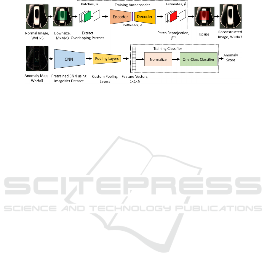
Figure 1: Block diagram of the proposed anomaly detection method (dashed lines show the steps involved in the training
step).
dimensionality and C, H, W represent the channels,
height, and width of the input image, respectively.
The overall process can be written as follows:
𝑥=𝐷𝐸
(
𝑥
)
=𝐷
(
𝑧
)
(1)
where z is the latent vector and 𝑥 the reconstruction
of the input. The functions 𝐸 and 𝐷 are
parameterized by CNNs.
For simplicity and computational speed, a per-
pixel error measure such as the L
loss is chosen to
force the AE to reconstruct its input:
𝐿
(
x,𝑥
)
=x
(
𝑐,ℎ,𝑤
)
−𝑥
(
𝑐,ℎ,𝑤
)
(2)
where x
(
𝑐,ℎ,𝑤
)
denotes the intensity value of image
x at the pixel
(
𝑐,ℎ,𝑤
)
. During evaluation, the per-
pixel ℓ
-distance of x and 𝑥 is compute to obtain a
residual map R
(
x,𝑥
)
∈ ℝ
××
.
For the AD task, AE is only trained on defect-free
samples. During the test, the AE is failed to
reconstruct defects that have not been seen during the
training. The reconstruction error, 𝐿
, of each test
data is then regarded as the anomaly score. Finally,
the data with a high anomaly score is defined as
anomalies.
There are two main issues for deploying AE for
the AD task in an industrial inspection scenario
including the high-resolution images and poor
performance due to simple per-pixel comparisons and
imperfect reconstructions (Bergmann et al., 2019b;
Nalisnick et al., 2018). In this paper, we address the
high resolution image issue by applying overlapping
patches along with conditional learning for AE,
which is discussed in this sub-section. In addition, we
propose a new approach to incorporate transfer
learning with the AE to avoid computing anomaly
scores using simple per-pixel comparisons, which is
discussed in the next sub-section.
We use downsizing and patch extraction to
resolve the high-resolution image problem for AE
modeling. It is assumed here that by downsizing the
input image to some extent, its normality (i.e. the
image details that represent normal class) are
preserved. After downsizing the input image,
overlapping patches are extracted to train the AE.
Together with the patches, the number of the patches
in the image (i.e. the patches’ location) is given to the
network as a conditional variable. The idea is to feed
both local (patches) and global (conditions)
information at the same time to the AE. The
conditional variables help the AE network to train
more efficiently and also to avoid reproducing small
defects given a defective test image to the network.
For anomaly map calculation given a test image, the
procedure is to apply the patch reprojection and
upsizing of the AE’s output. The anomaly map is then
obtained using the difference of the input and
reconstructed image.
The most common architecture utilized for AE in
AD is the convolutional layers followed by the
pooling layers and the fully connected layers in the
encoder side, and fully connected layers followed by
the convolutional layers and up-sampling in the
decoder side (Ribeiro et al., 2018). It is not
recommended to use convolutional layers without
dense layers for the AD task, because this type of
network is able to memorize the spatial information
of input and is somehow able to reconstruct the
defects given the test image. AE deploying only
convolutional layers fits better for other applications
like image segmentation and compression in which
detailed spatial information is very important for
encoding (Badrinarayanan et al., 2017; Yildirim et al.,
2018).
VISAPP 2022 - 17th International Conference on Computer Vision Theory and Applications
88
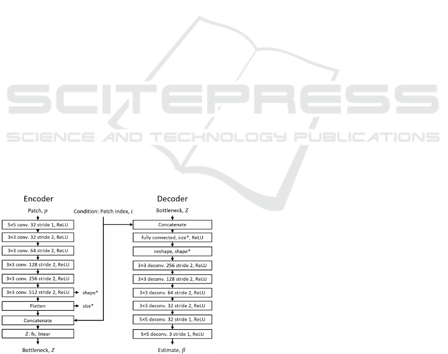
The proposed architecture for CPCAE is shown in
Figure 2. We utilize convolutional layers with the
stride in the encoder side and convolutional transpose
layers with the stride on the decoder side. The
convolutional (transpose) layers with the stride allow
the network to learn spatial subsampling (up-
sampling) from data, leading to a higher capacity of
transformation. In addition, we use concatenation in
the encoder part of AE to incorporate the new
conditional variable (the index of the patches, i.e.
patches’ number divided by total number of patches)
into our model. Similarly, the decoder is also
concatenated with the conditional vector.
The proposed CPCAE generates anomaly maps
to be used for training a one-class classifier in the
second step of the proposed hybrid method. The
challenge here is how to train the one-class classifier
using the training set already applied for the AE
training. One way to address this issue is to split the
training set into two parts to be separately used for
each step. However, since the training set in some
cases including the current project is too small,
splitting would decrease AE’s capability to learn
normal behavior. Another way is to train an AE using
sparse information of the training set to avoid
network overfitting and to preserve enough
information in anomaly maps for the classifier
training.
For a sparse autoencoder, in most cases, the loss
function is constructed by penalizing activations of
hidden layers so that only a few nodes can activate
when a single sample is fed into the network. 𝐿
and
𝐿
regularizations are widely used in deep learning,
and the main difference between them is that 𝐿
regularization tends to reduce the penalty
Figure 2: The architecture of proposed CPCAE for anomaly
map generation.
coefficients to zero, while 𝐿
regularization would
move coefficients near zero. More details can be
reached here (Chang et al., 2019). The loss function
using 𝐿
regularization is selected here as follows:
𝐿𝑜𝑠𝑠 = 𝐿
(
x,𝑥
)
+𝜆𝑎
()
(3)
the second term penalizes the absolute value of the
vector of activations 𝑎 in layer ℎ for sample 𝑖. A
hyperparameter 𝜆 is also used to control its effect on
the whole loss function.
3.2 Deep Feature-based
One-class Classification
In this sub-section, the second step of the proposed
method which involves feature extraction using a pre-
trained CNN model followed by a one class classifier
is explained. Specifically, the anomaly maps
generated using AE in the first step, are used to train
a one class classifier as shown in Figure 1. Using the
binary classification on top of the AE result, we
would like to leverage the transfer learning through
feature extraction via a pre-trained CNN network and
to avoid computing anomaly scores using simple per-
pixel comparisons of AE. The performance of many
supervised computer vision algorithms is improved
by transfer learning (Kornblith et al., 2019; Burlina et
al., 2019), i.e. by using discriminative embeddings
from the pre-trained networks. This is also true for
semi-supervised AD tasks as recent works suggest
that these feature spaces together with a one class
classifier outperform AE-based approaches (Nazaré
et al., 2018).
The second step of the proposed AD method takes
a set of anomaly maps generated by AE, 𝑋
=
𝑥
,𝑥
…𝑥
. It uses a pre-trained feature extractor
pre-trained on the Imagenet dataset, 𝐹 to extract
features from the entire training set, 𝑓
=𝐹
(
𝑥
)
. The
training set is now summarized as a set of embeddings
𝐹
= 𝑓
,𝑓
…𝑓
. The choice of deep network and
its depth are data-related and should be selected
experimentally. In this study, we use Xception
network just before the global pooling layer (Chollet,
2017). Xception can be considered as an extreme
Inception architecture (Szegedy et al., 2016), which
introduces the idea of depthwise separable
convolution. More mathematical details can be
reached here (Chollet, 2017). The global max pooling
layer is usually used on top of the last convolutional
layer of pre-trained networks to generate feature
embedding (Nazaré et al., 2018). Here, we apply a
new pooling layer to generate final image embedding
as shown in Figure 3. Since we feed the input image
Anomaly Detection for Industrial Inspection using Convolutional Autoencoder and Deep Feature-based One-class Classification
89
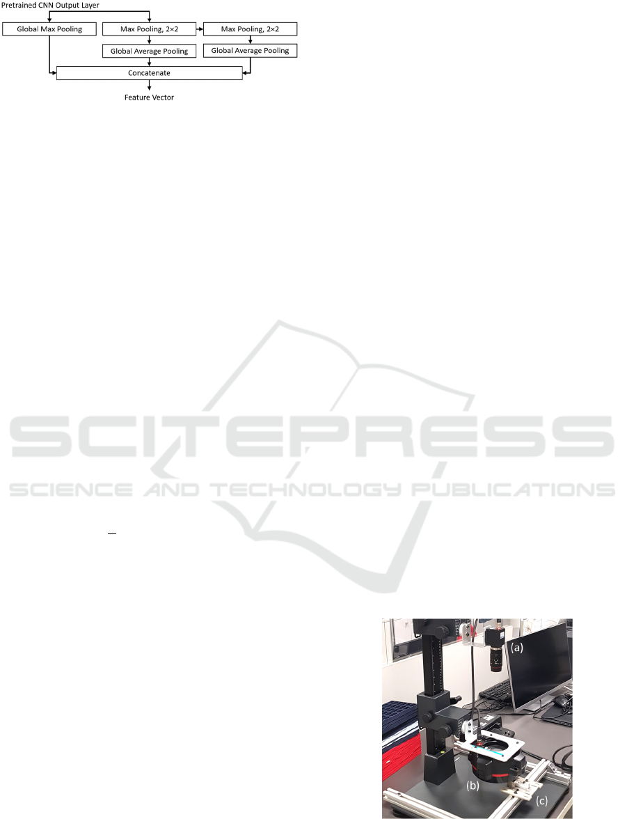
Figure 3: Proposed pooling layer used on top of the pre-
trained CNN network for feature extraction.
without downsizing into the pre- trained network, the
number of features after a global max-pooling layer are
very small to represent a high-resolution image. Using
the new pooling layer which consists of parallel and
cascade pollings along with concatenation, we have
three times more features as compared to the traditional
way to generate final embedding.
Having the image embedding after normalization
(mean removal and variance scaling), a suitable one-
class classifier such as one-class SVM (Scholkopf et
al., 2001), SVDD (Tax et al., 2004), or k-NN
(Bergman et al., 2020), can be trained on the
embeddings. In this study, k-NN is chosen as the
classifier which is widely applied for AD tasks
(Bergman et al., 2020; Nazaré et al., 2018; Guo et al.,
2018). The advantage of k-NN-based approaches is
that they do not need an assumption for the data
distribution and can be applied to different data types.
To detect if a new sample 𝑦 is anomalous, we first
extract its feature embedding using (7) and normalize
it. We then compute its k-NN distance and use it as
the anomaly score as follows:
𝑑
(
𝑦
)
=
1
𝑘
𝑓
−
𝑓
∈
(4)
𝑁
𝑓
denotes the 𝑘 nearest embeddings to 𝑓
in the
training set 𝐹
. Euclidean distance is used here that
often achieves superior results on features extracted
by deep networks (Bergman et al., 2020), but other
distance measures can be similarly used. We
determine if an image 𝑦 is normal or anomalous by
confirming if the distance 𝑑(𝑦) is larger than a
threshold.
4 EXPERIMENTAL RESULTS
AND DISCUSSION
In this Section, the results of the proposed method for
the AD task is presented. In addition, it is discussed
how to collect data for zipper cursors and evaluate the
proposed framework as well as several state-of-the-
art approaches. In the following sub-sections, we
discuss the following: experimental setup, dataset,
evaluation metrics, evaluated methods, and AD
results.
4.1 Experimental Setup
The IAS used here is a CV-X series vision system
from KEYENCE, which is a multi-modes IAS. The
model for the camera, lens, and lighting system are as
follows: CA-H200MX, CA-LHR50, and CA-
DRM10X. We use a 2-megapixel camera that
generates images with 1600×1200 size. In the current
IAS system setup, we use a diffused ring light system
near to the object in which the object is illuminated
from a low angle by uniform diffuse light through the
light conduction plate. The IAS together with the
camera and lighting stand with fixture and holder is
shown in Figure 4.
4.2 Dataset
The zipper cursor dataset including six different types
selected here is summarized in Table 1. The
anomalies manifest themselves in the form of bubble,
residue, halo, and scratches. In addition to zipper
cursor dataset, we evaluate the proposed method on
the MVTec dataset (Bergmann et al., 2019a). The
MVTec dataset comprises 15 categories, however, we
only consider 8 of 15 categories, which have rigid
shapes that can be registered. Table 2 gives an
overview of each object’s category. The anomalies
consist of different types of defects such as scratches,
dents, contaminations, and various structural
changes. For all datasets, pixel values of all images
are normalized to [0, 1], and the images are cropped
to maximize the field of view. Figure 5 shows
different sets of zipper cursors and different
categories of MVTec datasets used for the analysis.
Figure 4: Image acquisition setup, (a) CV-X series vision
system from KEYENCE, (b) Lighting system, and (c)
Holder and fixture.
VISAPP 2022 - 17th International Conference on Computer Vision Theory and Applications
90
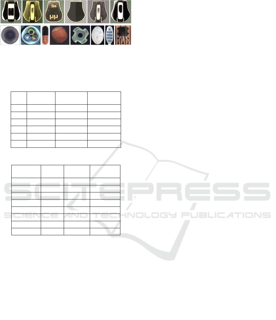
Figure 5: Anomaly detection dataset, first row, left to right:
zipper cursor dataset sets. #1 to #6. bottom row, left to right:
“Bottle”, “Cable”, “Capsule”, “Hazelnut”, “Metal Nut”,
“Pill”, “Toothbrush”, and “Transistor”.
Table 1: Statistical overview of the zipper cursor dataset.
Set # Train # Test
(normal)
# Test
(defective)
# 1 60 55 148
# 2 60 47 84
# 3 49 33 14
# 4 40 39 36
# 5 44 19 31
# 6 28 23 18
Table 2: Statistical overview of the MVTec AD dataset.
Set # Train # Test
(normal)
# Test
(defective)
Bottle 209 20 63
Cable 224 58 92
Capsule 219 23 109
Hazelnut 391 40 70
Metal Nut 220 22 93
Pill 267 26 141
Toothbrush 60 12 30
Transistor 213 60 40
4.3 Evaluation Metrics
Receiver operator characteristic (ROC) and
precision-recall (PR) curves are common metrics for
AD tasks which are defined over all possible decision
thresholds. It is also useful to quantitatively evaluate
the model performance using a single value rather
than comparing curves. The area under the ROC
curve (AUC) and average precision (AP) are the
common metrics that are obtained using ROC and PR
curves, respectively. AP summarizes a PR curve by a
sum of precisions at each threshold, multiplied by the
increase in recall, which is an approximation of the
area under the PR curve. Since AD task always has a
large skew in the class distribution, AP gives a more
accurate assessment of an algorithm’s performance
(Davis and Goadrich, 2006). In our experiments,
ROC curve, AUC, and AP were used to evaluate the
performance.
4.4 Evaluated Methods
We compare the proposed AD method with four
different approaches including AE (Bergmann et al.,
2019a), deep feature one class classifier (Perera and
Patel, 2019), variation (Steger et al., 2018) and
nearest neighbor (NN) approaches (Vaikundam et al,
2016). For the evaluation of the AE method, we use
the same AE architecture described in the paper for
the proposed method. For deep feature one classifier,
we use the implementation proposed in (Perera and
Patel, 2019), which applied a pre-trained CNN
network to the image and extract features using global
max pooling. After normalization, k-NN is used to
generate anomaly scores ( 𝑘=15 is used for
classifier). The variation is a baseline method, which
is based on statistics, mean and standard deviation,
computed from the normal training set. Anomaly
maps are then obtained by computing the distance of
each test pixel’s gray value to the computed pixel
mean relative to the computed standard deviation.
The anomaly score is obtained using the sum of
squares of pixels in the anomaly map. NN is another
baseline method in which the anomaly score is
obtained by computing the distance (usually 𝑙
)
between the test sample and its most similar image
inside the normal training set. It should be mentioned
that parameters tuning is performed for different
models included in the comparison to find the best
solution for them. Apart from the methods that have
been implemented for comparison, we also report
AUC results for the MVTec dataset from recently
published deep-learning-based methods consisting of
GeoTrans (Golan et al., 2018), GANomaly (Akcay et
al., 2018), VAE (Jinwon and Sungzoon, 2019),
AnoGAN (Schlegl et al., 2017), and AE applying
structural similarity index measure (SSIM)
(Bergmann et al., 2019b), taken directly from (Chao-
Qing et al., 2019) and (Bergmann et al., 2020).
4.5 Anomaly Detection Results
The first experiment is the two-dimensional tSNE
visualizations of the extracted features from the
anomaly maps as compared to the AE’s latent space
variables for normal and anomalous images in the test
set (Van der Maaten and Hinton, 2008). AE’s latent
space variables are also being used as image
embedding for AD in recent years (Kawachi et al.,
2018; Guo et al., 2018; Amarbayasgalan et al., 2018).
The tSNE visualizations are shown in Figure 6 for
zipper cursor and MVTec datasets. Qualitatively,
features extracted by the proposed method facilitate
better distinction between normal and anomalous
Anomaly Detection for Industrial Inspection using Convolutional Autoencoder and Deep Feature-based One-class Classification
91
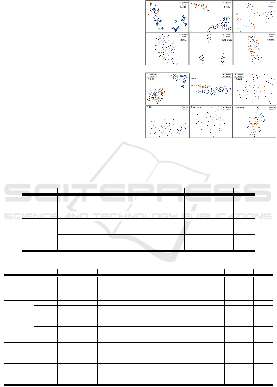
images as compared to the AE’s latent space
variables.
The second experiment presents the AD results of
the proposed method as well as the baselines and
deep-learning based approaches for zipper cursors
and MVTec datasets. Tables 3 and 4 show AUC and
AP metrics, and Figures 7 and 8 show the ROC
curves. It can be seen from the results that the
proposed hybrid framework outperformed state-of-
the-art methods in terms of different metrics,
specifically PR, which gives a more accurate picture
of an algorithm’s performance when there is a large
skew in the class distribution (Davis and Goadrich,
2006). The second best method on average is AE for
the zipper cursor dataset and deep feature
classification for the MVTec dataset. This is because
AE is able to generalize better on the zipper cursor
dataset which has simpler appearances as compared
to the MVTec dataset. The baseline approaches
including variation and NN methods could not
produce reliable results. In addition, the proposed
method outperformed recently published deep
learning-based methods in terms of AUC metric for
the MVTec dataset as shown in Table 4.
(a)
(b)
Figure 6: 2D t-SNE plots of the feature embedding obtained
using (a) the AE’s latent space representation and (b)
proposed embedding for different datasets, which are
mentioned in the corner of each plot.
Table 3: Anomaly detection results for the zipper cursor dataset.
Methods Metrics Set #1 Set #2 Set #3 Set #4 Set #5 Set #6 Mean
Proposed
AUC 95.67 96.90 95.20 88.08 94.64 96.10 94.43
AP 98.35 98.16 90.90 88.81 96.00 96.43 94.77
AE (L
2
)
AUC 87.81 95.59 92.21 77.54 78.48 91.11 87.12
AP 95.24 97.05 87.88 83.01 82.47 90.17 89.30
Deep Feature
AUC 85.32 95.77 80.81 74.97 62.15 93.77 82.13
AP 93.78 96.99 51.10 74.75 73.47 93.31 80.56
NN
AUC 91.06 94.14 90.69 82.72 76.31 91.58 87.75
AP 96.36 96.50 86.51 85.94 79.88 92.83 89.67
Variation
AUC 91.32 93.45 91.13 77.06 73.53 81.76 84.70
AP 96.18 95.47 86.37 83.33 77.11 81.06 86.58
Table 4: Anomaly detection results for the MVTec dataset.
Methods Metrics Bottle Cable Ca
p
sule Hazelnut Metal Nut Pill Toothbrush Transisto
r
Mean
Proposed
AUC 99.71 87.73 86.39 95.87 79.28 86.74 100.0 93.06
91.09
AP 99.90 92.54 96.71 97.90 94.88 97.23 100.0 91.68
96.35
AE (L
2
)
AUC 89.77 82.70 54.89 85.23 59.45 79.85 76.68 86.35
75.31
AP 96.83 89.70 87.12 91.74 87.36 95.59 91.03 85.72
91.39
Deep Feature AUC 96.71 83.61 88.37 90.29 68.93 71.71 91.67 85.33 83.27
AP 98.90 90.45 96.40 95.01 90.21 92.38 96.85 85.51 93.89
NN
AUC 81.02 81.30 69.78 52.83 60.16 63.66 95.84 81.12 68.12
AP 93.78 88.11 91.09 74.29 87.76 88.71 98.46 78.64 87.29
Variation
AUC 79.25 68.20 46.05 49.13 42.95 62.86 86.48 73.09 58.07
AP 93.12 77.88 83.08 70.93 79.20 87.56 94.36 75.15 81.96
GeoTrans AUC 74.4 78.3 67.0 63.0 35.9 63.0 97.2 86.9 63.60
AP * * * * * * * * *
GANomaly AUC 89.2 75.7 73.2 74.3 78.5 74.3 65.3 79.2 77.53
AP * * * * * * * * *
VAE AUC 89.7 65.4 52.6 87.8 57.6 76.9 69.3 62.6 71.66
AP * * * * * * * * *
AnoGAN AUC 62.0 38.3 30.6 69.8 32.0 77.6 74.9 54.9 51.71
AP * * * * * * * * *
AE (SSIM) AUC 83.4 47.8 86.0 91.6 60.3 83.0 78.4 72.5 75.35
AP * * * * * * * * *
VISAPP 2022 - 17th International Conference on Computer Vision Theory and Applications
92
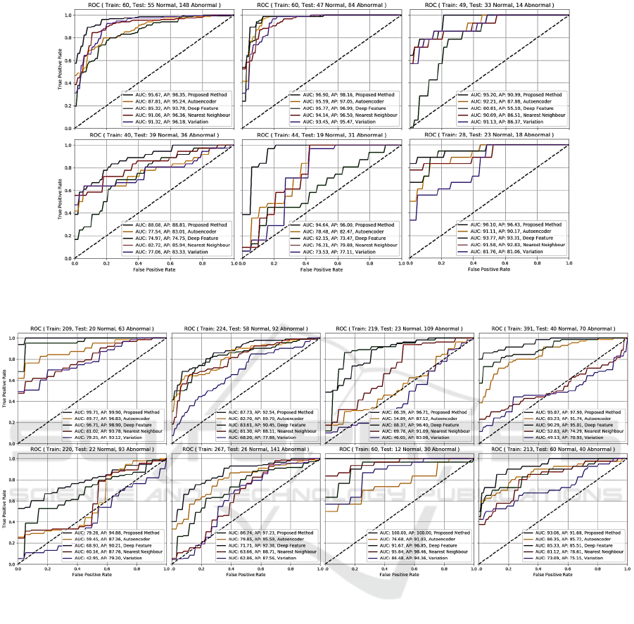
Figure 7: Comparison of ROC curves obtained for different methods and datasets, (top row, left to right): sets #1-3, (bottom
row, left to right): sets #4-6 of zipper cursor dataset.
Figure 8: Comparison of ROC curves obtained for different methods and datasets, (top row, left to right): Bottle, Cable,
Capsule, Hazelnut, (bottom row, left to right): Metal Nut, Pill, Toothbrush, Transistor of MVTec dataset.
For the zipper cursor dataset where there are not
enough samples for training, e.g. sets #4-6, the
performance of the proposed method along with other
approaches decline. For the MVTec dataset, good
performance can be observed on the “bottle”,
“toothbrush”, “hazelnut”, and “transistor”, while it
yields comparably poorer results for “metal nut”,
“cable”, and “pill”. This is because the latter objects
contain certain random variations on the objects’
surfaces, which prevents the model from learning
detailed information for most of the image pixels.
For the final experiment, we demonstrate the
reconstructed images and anomaly maps generated
using the proposed CPCAE method for some samples
of zipper cursor shown in Figure 9, and MVTec
datasets illustrated in Figure 10. For the zipper cursor
dataset, anomalies manifest themselves in the
different types of defects such as bubble, residue,
scratch, and halo as shown in Figure 9 (b), and for the
MVTec dataset, anomalies are consisting of broken,
crack, cut, color, contamination, and misplaced as
illustrated in Figure 10 (b). It can be seen from the
results that the proposed method fails to reconstruct
the defected regions, while it can generalize well to
reconstruct the normal unseen images within normal
specification ranges.
Anomaly Detection for Industrial Inspection using Convolutional Autoencoder and Deep Feature-based One-class Classification
93
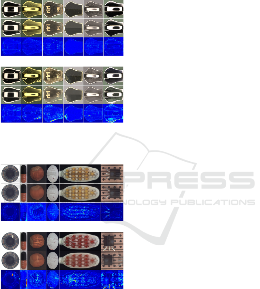
(a)
(b)
Figure 9: Anomaly detection results for (a) normal and (b)
defected samples, top to bottom: input image, reconstructed
image using AE, and anomaly map; left to right, sets #1 to
#6 of zipper cursor dataset.
(a)
(b)
Figure 10: Anomaly detection results for (a) normal and (b)
defected samples, top to bottom: input image, reconstructed
image using AE, and anomaly map; left to right, “Bottle”,
“Capsule”, “Hazelnut”, “Pill”, “Toothbrush” and
“Transistor” of MVTec dataset.
5 CONCLUSIONS AND FUTURE
WORKS
A novel framework for the semi-supervised anomaly
detection tasks is proposed here to introduce a method
for zipper cursors’ visual inspection. The proposed
method uses a conditional path-based convolutional
autoencoder to tackle the challenges related to the
high-resolution images in industrial inspection
scenarios. In addition, we use a binary classification
on top of the autoencoder result to leverage the
transfer learning through feature extraction via a pre-
trained CNN network and to avoid computing
anomaly scores using the simple per-pixel
comparisons of autoencoder. We demonstrate state-
of-the-art performance on different datasets,
including the zipper cursor dataset and the recently
introduced MVTec dataset.
For future work, we investigate other types of
deep learning frameworks, e.g. variational
autoencoder and generative adversarial network
instead of autoencoder applied in the proposed
method. In addition, regarding deep feature one-class
classification, we would like to explore different one-
class classifiers to improve the results.
ACKNOWLEDGEMENTS
This work has been supported by the Swiss
Innovation Agency (Innosuisse) project 27371.1 IP-
ICT. The authors would like to thank RIRI SA for
their assistance in preparing zipper cursor datasets
and their valuable feedback.
REFERENCES
Akcay, S., Atapour-Abarghouei, A., and Breckon, T. P.
(2018). GANomaly: Semi-Supervised Anomaly
Detection via Adversarial Training. In ACCV.
Andrews, J.T.A., Tanay, T., Morton, E.J., and Griffin, L.D.
(2016). Transfer Representation Learning for Anomaly
Detection. In Anomaly Detection Workshop at ICML.
Badrinarayanan V., Kendall A. and Cipolla R. (2017).
SegNet: A Deep Convolutional Encoder-Decoder
Architecture for Image Segmentation. IEEE
Transactions on Pattern Analysis and Machine
Intelligence, 39 (12): 2481-2495.
Baklouti, R., Mansouri, M., Nounou, M., Nounou, H., and
Hamida, A.B. (2016). Iterated robust kernel fuzzy
principal component analysis and application to fault
detection. Journal of Computational Science 15: 34–49
VISAPP 2022 - 17th International Conference on Computer Vision Theory and Applications
94

Bergman, L., Cohen, N., and Hoshen, Y. (2020). Deep
Nearest Neighbor Anomaly Detection. ArXiv,
abs/2002.10445.
Bergmann, P., Fauser, M., Sattlegger, D., and Steger, C.
(2019a). MVTec AD - A Comprehensive Real-World
Dataset for Unsupervised Anomaly Detection. IEEE
Conference on Computer Vision and Pattern
Recognition (CVPR), pages 9592-9600.
Bergmann, P., Fauser, M., Sattlegger, D., and Steger, C.
(2020). Uninformed students: Student-teacher anomaly
detection with discriminative latent embeddings. In
CVPR.
Bergmann, P., Lowe, S., Fauser, M., Sattlegger, D., and
Steger, C. (2019b). Improving Unsupervised Defect
Segmentation by Applying Structural Similarity to
Autoencoders. In Proceedings of the 14
th
International
Joint Conference on Computer Vision, Imaging and
Computer Graphics Theory and Applications, volume
5, pages 372–380
Breunig, M., Kriegel, H., Ng, R.T., Sander, J. (2000). LOF:
identifying density-based local outliers. International
Conference on Management of Data (SIGMOD), pages
93-104
Burlina, P., Joshi, N., and Wang, I. (2019). Where’s Wally
Now? Deep Generative and Discriminative
Embeddings for Novelty Detection. IEEE Conference
on Computer Vision and Pattern Recognition (CVPR),
pages 11507-11516
Chang, S., Du, B., and Zhang, L., (2019). A Sparse
Autoencoder Based Hyperspectral Anomaly Detection
Algorithm Using Residual of Reconstruction Error.
IEEE International Geoscience and Remote Sensing
Symposium, pages 5488-5491
Chao-Qing, H., et al. (2019). Inverse-Transform
AutoEncoder for Anomaly Detection.” ArXiv
abs/1911.10676.
Chollet, F. (2017). Xception: Deep Learning with
Depthwise Separable Convolutions. IEEE Conference
on Computer Vision and Pattern Recognition (CVPR),
pages 1800-1807
Davis, J., and Goadrich, M. (2006). The relationship
between precision recall and ROC curves. In
International Conference on Machine Learning
(ICML), pages 233–240
Deng, J. et al. (2009). Imagenet: A large-scale hierarchical
image database. IEEE Conference on Computer Vision
and Pattern Recognition CVPR. pages 248–255.
Eskin, E. (2000). Anomaly detection over noisy data using
learned probability distributions. In Proceedings of the
17th International Conference on Machine Learning,
pages 255-262.
Golan, I., and El-Yaniv, R. (2018). Deep anomaly detection
using geometric transformations. In NeurIPS.
Guo, J., Liu, G., Zuo, Y. and Wu, J. (2018). An Anomaly
Detection Framework Based on Autoencoder and
Nearest Neighbor. 15th International Conference on
Service Systems and Service Management (ICSSSM),
pages 1-6
Harrou, F., Kadri, F., Chaabane, S., Tahon, C., Sun, Y.
(2015). Improved principal component analysis for
anomaly detection: Application to an emergency
department. Computers & Industrial Engineering 88:
63–77
Jinwon, An., and Sungzoon, Cho. (2015). Variational
Autoencoder based Anomaly Detection using
Reconstruction Probability. SNU Data Mining Center,
Tech. Rep. Special Lecture on IE 2:1–18
Kawachi, Y., Koizumi, Y., and Harada, N. (2018).
Complementary set variational autoencoder for
supervised anomaly detection. IEEE International
Conference on Acoustics, Speech and Signal
Processing (ICASSP), pages 2366–2370.
Kingma, D. P., Welling, M. (2014). Auto-Encoding
Variational Bayes. International Conference on
Learning Representations (ICLR), pages 1-14
Kornblith, S., Shlens, J., and Le, Q. V. (2019). Do better
imagenet models transfer better? IEEE Conference on
Computer Vision and Pattern Recognition (CVPR),
pages 2661-2671.
Krizhevsky, A., and Hinton, G. (2009). Learning multiple
layers of features from tiny images. Technical Report.
University of Toronto.
LeCun, Y. (1998). The mnist database of handwritten
digits. http://yann. lecun. com/exdb/mnist/
Matsubara, T., Hama, K., Tachibana, R., and Uehara, K.
(2018). Deep generative model using unregularized
score for anomaly detection with heterogeneous
complexity. arXiv preprint arXiv:1807.05800.
Nalisnick, E., Matsukawa, A., Whye The, Y., Gorur, D.,
and Lakshminarayanan, B. (2018). Do Deep Generative
Models Know What They Don’t Know? arXiv preprint
arXiv:1810.09136.
Napoletano, P., Piccoli, F., and Schettini, R. (2018).
Anomaly Detection in Nanofibrous Materials by CNN-
Based Self-Similarity. Sensors, 18 (1): 209
Nazaré, S. et al. (2018). Are pre-trained CNNs good feature
extractors for anomaly detection in surveillance
videos?” ArXiv abs/1811.08495.
Olive, D.J. (2017). Principal Component Analysis, Robust
Multivariate Analysis, Springer: 189–217.
Oza, P. and Patel, V. M. (2019). One-Class Convolutional
Neural Network. IEEE Signal Processing Letters, 26
(2): 277-281.
Perera, P., and Patel, V. M., (2019). Learning Deep
Features for One-Class Classification. IEEE
Transactions on Image Processing, 28 (11): 5450-5463.
Pol, A., Berger, V., Germain, C., Cerminara, G., and
Pierini, M., (2019). Anomaly Detection with
Conditional Variational Autoencoders. IEEE
International Conference On Machine Learning and
Applications (ICMLA), pages 1651-1657
Ribeiro, M., Lazzaretti, A. E., and Lopes, H. S. (2018). A
study of deep convolutional auto-encoders for anomaly
detection in videos. Pattern Recognition Letters, 105:
13-22,
Ruff, L., Görnitz, N., Deecke, L., Siddiqui, S.,
Vandermeulen, R.A., Binder, A., Müller, E., and Kloft,
M. (2018). Deep One-Class Classification. In
Proceedings of the 35th International Conference on
Machine Learning, volume 80, pages 4393-4402
Anomaly Detection for Industrial Inspection using Convolutional Autoencoder and Deep Feature-based One-class Classification
95

Saeedi, J., Dotta, M., Galli, A. et al. (2021). Measurement
and inspection of electrical discharge machined steel
surfaces using deep neural networks. Machine Vision
and Applications 32, 21: 1-15
Schlegl, T., Seebock, P., Waldstein, S. M., Erfurth, U. S.,
and Langs, G. (2017). Unsupervised Anomaly
Detection with Generative Adversarial Networks to
Guide Marker Discovery. In International Conference
on Information Processing in Medical Imaging, pages
146–157.
Scholkopf, B., Platt, J.C., Shawe-Taylor, J.C., A.J. Smola,
and R.C. Williamson. (2001). Estimating the support of
a high-dimensional distribution. Neural Computing,
13(7): 1443–1471.
Steger, C., Ulrich, M., and Wiedemann, C. (2018). Machine
Vision Algorithms and Applications. Wiley-VCH,
Weinheim, 2
nd
edition.
Szegedy, C., Vanhoucke, V., Ioffe, S., et al. (2016).
Rethinking the Inception Architecture for Computer
Vision. In Proceedings of the IEEE Computer Society
Conference on Computer Vision and Pattern
Recognition, pages 2818–2826
Tang, B., He, H. (2017). A local density-based approach for
outlier detection, Neurocomputing, 241: 171–180
Tax, D.M.J., and Duin, R.P.W. (2004). Support vector data
description. Mach. Learn., 54(1): 45–66.
Vaikundam, S., Hung, T., and Chia, L.T. (2016). Anomaly
region detection and localization in metal surface
inspection. IEEE International Conference on Image
Processing (ICIP), pages 759-763
Van der Maaten, L. and Hinton, G. E. (2008). Visualizing
high-dimensional data using t-SNE. Journal of
Machine Learning Research 9:2579–2605
Xiao, H., Rasul, K., and Vollgraf, R. (2017). Fashion-mnist:
a novel image dataset for benchmarking machine
learning algorithms. arXiv preprint arXiv:1708.07747.
Xu, H., Caramanis, C., and Sanghavi, S. (2012). Robust
PCA via outlier pursuit. IEEE Transactions on
Information Theory, 58 (5): 3047-3064
Yildirim, O., Tan, R.S., Acharya, U. R., (2018). An
efficient compression of ECG signals using deep
convolutional autoencoders, Cognitive Systems
Research, volume 52, pages 198-211
VISAPP 2022 - 17th International Conference on Computer Vision Theory and Applications
96
