
Random-walk Segmentation of Nuclei in Fluorescence Microscopic
Images with Automatic Seed Detection
Tabea Margareta Grace Pakull, Frederike Wirth and Klaus Brinker
Hamm-Lippstadt University of Applied Sciences, Marker Allee 76-78, 59063 Hamm, Germany
Keywords:
Medical Image Analysis, Computer Vision, Fluorescence Microscopy, Cell Nuclei Segmentation,
Random-walk Segmentation.
Abstract:
In personalized immunotherapy against cancer analysis of cell nuclei in tissue samples can provide helpful
information to predict whether the benefits of the therapy outweigh the usually severe side effects. Since
segmentation of nuclei is the basis for all further analyses of cell images, research into suitable methods is
of particular relevance. In this paper we present and evaluate two versions of a segmentation pipeline based
on the established random-walk method. These versions contain automatic seed detection, using a distance
transformation in one of them. In addition, we present a method to select the required hyper-parameter of
the random-walk algorithm. The evaluation using a benchmark dataset shows that promising results can be
achieved with respect to common evaluation metrics. Furthermore, the segmentation accuracy can compete
with a reference CellProfiler segmentation pipeline, based on the watershed transformation. Based on the
presented pipeline, the random-walk method can also be integrated into more advanced pipelines to further
improve segmentation results.
1 INTRODUCTION
With 10 million deaths caused by cancer in 2020, it
is one of the most common causes of death world-
wide (World Health Organization, 2021). In the fight
against cancer, immunotherapy has become a promis-
ing treatment option by using the body’s immune sys-
tem to fight cancer (Esfahani et al., 2020). The dis-
covery of immune checkpoint inhibitors, which pre-
vent tumor cells from using immune escape mecha-
nisms, was of great importance for research.
There is still insufficient research into which peo-
ple benefit from this kind of treatment. A preselection
is particularly important because the side effects can
be severe and even fatal (Esfahani et al., 2020). As
part of the ImmunePredict research project, we aim
at improving this selection by developing a predic-
tive model based on fluorescence microscopy imag-
ing. The first step in analyzing the images is to seg-
ment nuclei to accumulate cellular information for
predicting treatment success in further steps.
For segmentation, different methods were pro-
posed, that can be divided into the categories of
optimization, threshold and machine-learning-based
methods (Abdolhoseini et al., 2019). The latter is usu-
ally considered state-of-the-art and produce promis-
ing results for nuclei segmentation (cf. Liu et al.,
2021; Zaki et al., 2020; Kowal et al., 2020). Neverthe-
less, segmentation of nuclei remains challenging. For
example, overlapping nuclei are typically segmented
less accurately. A common approach is to use hybrid
methods by combining multiple techniques. The wa-
tershed transformation, which was evaluated as a part
of our research project (Wirth et al., 2020), for exam-
ple, can be combined with threshold and model-based
methods (Abdolhoseini et al., 2019) or used for post-
processing (Kowal et al., 2020), to improve segmen-
tation of clustered cell nuclei.
The random-walk algorithm can be widely applied
for image processing (e.g. image fusion, registra-
tion and segmentation) and it has already been ap-
plied successfully for segmentation in the oncologi-
cal field (Wang et al., 2019). Besides the model we
use in this paper, proposed by Grady (2006), there are
alternating models to suit different use cases (Wang
et al., 2019). Key points in the improvement of the
algorithm are the preprocessing of input data and the
position of required seeds, that typically need user in-
teraction (Wang et al., 2017). An automatic solution
is necessary to make better use of the algorithm and
to combine it with e.g. deep learning methods.
The aim of this paper is to explore the basic po-
tential of the random-walk method for segmentation
of nuclei in fluorescence images by assessing the per-
formance of two pipeline versions we developed. We
follow an automatic approach by proposing two au-
Pakull, T., Wirth, F. and Brinker, K.
Random-walk Segmentation of Nuclei in Fluorescence Microscopic Images with Automatic Seed Detection.
DOI: 10.5220/0010780400003123
In Proceedings of the 15th International Joint Conference on Biomedical Engineering Systems and Technologies (BIOSTEC 2022) - Volume 2: BIOIMAGING, pages 103-110
ISBN: 978-989-758-552-4; ISSN: 2184-4305
Copyright
c
2022 by SCITEPRESS – Science and Technology Publications, Lda. All rights reserved
103
tomatic seed detection methods with appropriate pre-
processing for detection and the random-walk algo-
rithm itself, as well as a method to set the hyper-
parameter β (see (1)). This enables the use of our
pipeline separately or in combination with sophisti-
cated techniques.
This paper is organized as follows: We summarize
the concept of segmentation using the random-walk
method in section 2. After that we outline the im-
plementation of our pipeline in section 3, which we
evaluate using a publicly available dataset presented
in section 4 and the metrics listed in section 5. The
results are presented in section 6 followed by the dis-
cussion in section 7. We provide a summary of our
findings and concluding remarks in section 8.
2 RANDOM-WALK
SEGMENTATION
A random-walk is a stochastic process that can be
used to describe random movements (Grady, 2006).
For segmentation, the random-walk is considered in
at least two dimensions. It operates on an undirected
graph and has a bias, which means that the steps on
this graph have different probabilities represented as
edge weights (Grady, 2006).
The segmentation method used in this paper was
proposed by Grady (2006). Grady (2006) derived a
method for analytically computing the desired prob-
abilities without the need of a rather inefficient sim-
ulation of a random-walk. The result of this method
is an image that is segmented into regions that are as-
signed their own specific label. It is necessary to as-
sign labels to certain pixels (seeds) in advance. The
remaining pixels are assigned to these labels using the
random-walk algorithm by calculating the probability
that a random-walker that starts at a pixel will first
reach a seed with a certain label (Grady, 2006).
The algorithm is based on the conversion of the
image into a graph G = (V, E) that consists of nodes
v ∈ V and edges e ∈ E. To prevent the random-walker
from crossing sharp intensity gradients, the edges are
weighted with a weighting function. As described in
(Wang et al., 2019) different weighting functions have
been proposed. We use the Gaussian weighting func-
tion (see (1)) in our pipeline:
w(e
i, j
) = w
i, j
= e
−β(g
i
−g
j
)
2
(1)
The edge e
i, j
connects the neighboring nodes i
and j. β is the only free parameter in the algorithm.
The intensities of the pixels are denoted as g
i
and g
j
.
The probability with which the random-walker uses
an edge is referred to as w(e
i, j
). Thus, strong inten-
sity gradients yield small probabilities.
The required probabilities are determined by solv-
ing a sparse linear system of equations. For each node
a k-tuple vector x
i
= (x
1
i
, ..., x
k
i
) is computed. The final
segmentation is determined by assigning each node v
i
to the label corresponding to argmax(x
s
i
).
The algorithm always comes up with the same
unique result, which depends on the seed selection.
For completely black images or noise, the method
creates a so-called neutral segmentation. For each
seed, the segmented areas then resemble Voronoi cells
(Grady, 2006).
3 IMPLEMENTATION
Our proposed pipeline are based on methods of the
following standard python libraries: NumPy
1
, SciPy
2
,
OpenCV
3
, scikit-image
4
and pandas
5
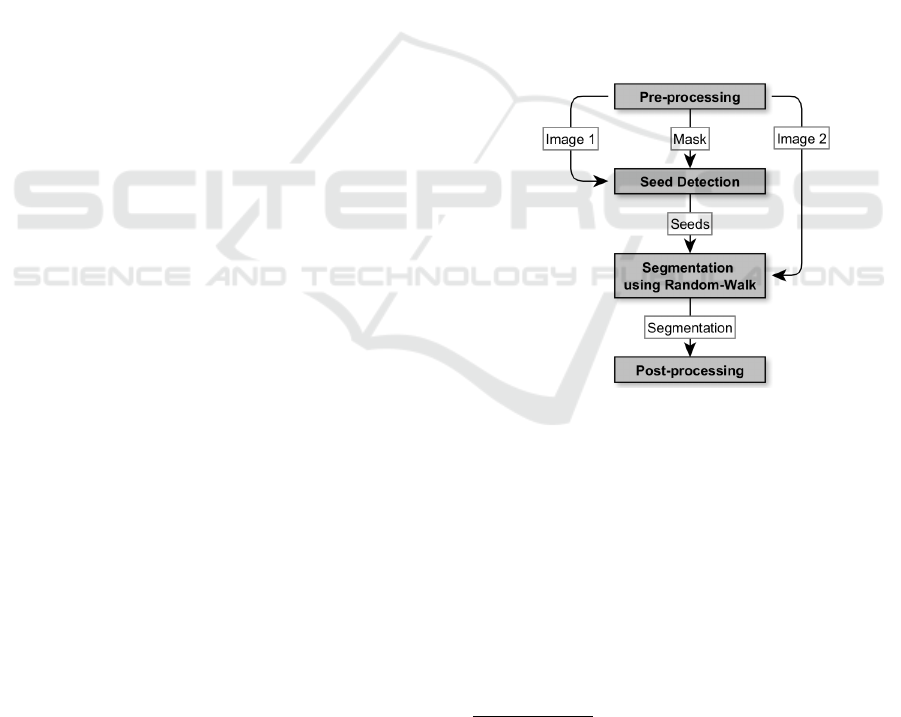
. Figure 1 shows
a schematic representation of our pipeline.
Figure 1: Schematic representation of the pipeline for seg-
mentation using the random-walk algorithm.
An image is taken from a dataset and prepro-
cessed. Since a distance transformation is optional
in the preprocessing step, there are two versions of
the pipeline, which, however, do not differ in the gen-
eral process. Preprocessing produces one image that
is used in seed detection and a second one that is used
for segmentation. In addition a mask seed detection
is created. As the first preprocessing step we reduce
noise in all of three images with the non-local-means
method, the contrast is optimized with the help of
an adaptive histogram equalization and edges are en-
1
https://numpy.org/ (version 1.18.5)
2
https://www.scipy.org/ (version 1.5.0)
3
https://opencv.org/ (version 4.5.1.48)
4
https://scikit-image.org/ (version 0.16.2)
5
https://pandas.pydata.org/ (version 1.0.5)
BIOIMAGING 2022 - 9th International Conference on Bioimaging
104

hanced by using a Sobel filter.
To create the mask we use the Li threshold (Li and
Lee, 1993) after that and then filter out small objects
to prevent detection of seeds for artifacts in the back-
ground. If the distance transformation is to be used
before seed detection, we apply the Li threshold on an
image with 1.5 times more enhanced edges, only us-
ing strong edges. After the transformation, a Gaussian
filter is applied and the intensity values get stretched
to cover values from 0 to 255. Without the transfor-
mation, only the last two steps are required after the
edge enhancement.
The image, to which the random-walk algorithm
is applied, demands a different preprocessing. Hence,
we use a background subtraction after noise reduction
and stretch the intensity values as described before.
Lastly, we dim intensity values to 40% of the maxi-
mum intensity to reduce contrast in bright regions.
In the developed pipeline, local maxima are used
as seeds. In order to avoid too many seeds per ob-
ject and yet not set an overall upper limit, only seeds
that are at least ten pixels apart are accepted. The
determined seeds are marked in a labeled image. In
addition, the biggest region of the background, after
dilating the objects in the mask from preprocessing,
is marked as a background seed. If a distance trans-
formation is used, the seeds for the nuclei are dilated
before labeling.
Using the random walker()-method of the scikit-
image library, a segmentation of the image is created.
As post-processing, objects that are larger than a pre-
defined value (here 5000) are removed from the image
and the biggest object is labeled as the background.
4 DATASET
The image dataset BBBC039v1
6
(Caicedo et al.,
2019), available from the Broad Bioimage Bench-
mark Collection (Ljosa et al., 2012), was used for
evaluating the two pipeline versions. The collection
was published by the Carpenter lab at the Broad Insti-
tute and contains sets of microscopic images. In ad-
dition, the sets contain a ground truth for each image
as well as metadata.
The metadata describes a division into training,
validation and test set consisted of 100, 50 and 50
images respectively. For this paper, these sets were
used as follows: The training dataset was used dur-
ing pipeline development. The validation dataset was
used to determine the β parameter. Finally, the test
dataset is used to evaluate the segmentation accuracy.
6
https://sites.broadinstitute.org/bbbc/BBBC039
4.1 Image Data
The BBBC039v1 image set contains 200 images in
which nuclei of cell line U2OS can be seen. The hu-
man osteosarcoma cell line U2OS was obtained from
a tumor in the tibia of a 15-year-old girl in 1964 (Ni-
forou et al., 2008). The images were acquired with a
fluorescence microscopy where the DNA was stained
with Hoechst. They have a resolution of 520 × 696
pixels and are stored as 16-bit TIFF files.
This dataset is rather challenging because of
strong intensity differences within and between the
nuclei. Some of them overlap or touch each other.
The size and shape of nuclei can differ due to a
wide variety of phenotypes, including micronuclei,
toroidal, fragmented, round and elongated nuclei
(Caicedo et al., 2019). The number of nuclei in an
image varies between 0 and 231. All images contain
some noise and a couple of images are almost entirely
filled with noise. In addition, some images contain
bright artifacts that cover up nuclei or cause strongly
reduced intensity values in surrounding areas. A to-
tal of approximately 23000 nuclei were manually seg-
mented by biologists for this dataset.
4.2 CellProfiler Pipeline
The Broad Institute has also published a reference
pipeline for the CellProfiler
7
software, which is a pos-
sible solution to the segmentation problem.
The preprocessing steps of this pipeline include
morphological operations, background subtraction
and applying a Sobel filter to enhance edges. A Gaus-
sian filter is applied to the image and a binary image is
created using a global Li threshold (Li and Lee, 1993).
Even though the typical diameter is specified with 20
to 80 pixels, objects outside these limits are not dis-
carded. Then, objects are identified that potentially
contain multiple nuclei. For these objects a distance
transformation is applied and the local maxima of its
output are used as seeds for a watershed transforma-
tion. All maxima that are less than ten pixels apart are
discarded. A smoothing filter is used to post-process
the segmentation to prevent over-segmentation. Fi-
nally, all holes in the objects are filled.
5 EVALUATION METRICS
Despite the importance of evaluating a segmentation
algorithm, there is no consensus on how it should be
7
https://cellprofiler.org/
Random-walk Segmentation of Nuclei in Fluorescence Microscopic Images with Automatic Seed Detection
105

done (Sonka et al., 2015). As part of the ImmunePre-
dict project, suitable evaluation metrics for supervised
evaluation were selected (Wirth et al., 2020). They
include pixel- and object-based methods. The ground
truth data in the BBBC039v1 dataset are used as ref-
erence (R) for the created segmentations (S).
5.1 Pixel-based Metrics
Pixel-based evaluation can be obtained through cal-
culation of the Rand Index (RI) (Rand, 1971) and
the Jaccard Index (JI) (Jaccard, 1901). They consider
whether pixels of pairs of pixel in R or S are assigned
to the same or to different objects. The intensities in
S are called S
i
and S
j
and R
i
and R
j
in R. All combi-
nations of pixels are considered as long as i 6= j. The
pairs are divided into the groups A to D according to
following scheme.
A: S
i
= S
j
∧ R
i
= R
j
C: S
i
= S
j
∧ R
i
6= R
j
B: S
i
6= S
j
∧ R
i
= R
j
D: S
i
6= S
j
∧ R
i
6= R
j
Groups A and D contain pixel pairs for which S
and R agree that pixels of the pair belong to the same
object or not. Conversely, groups B and C contain the
pairs for which there is no agreement in this respect.
The number of pairs in the corresponding groups are
denoted by a, b, c and d. Thus the RI is given by:
RI(R, S) =
a + d
a + b + c + d
=
a + d
n
2
. (2)
Here n denotes the total number of pixels in S and
R respectively. If S and R overlap completely, the in-
dex takes a value of 1. If there is less overlap, the
value is lower.
The above definition of a, b, c and d is also used
to calculate the JI:
JI(R, S) =
a + d
b + c + d
. (3)
The upper limit for JI depends on the number and
size of nuclei in relation to the image size. Thus, it
only allows a comparison between segmentations that
were created for the same data.
5.2 Object-based Metrics
For object-based metrics, reference objects in R must
be assigned to the objects in S. The object in R is de-
termined with which an object in S shares the most
pixels. On this basis, the maximum of the small-
est distance between two objects can be calculated,
which is called the Hausdorff Distance (HD). This can
be calculated as described by Coelho et al. (2009).
HD(R, S) = maxD(i) : S
i
6= R
i
(4)
Where D
i
is the minimum distance of a pixel i on
the object boundary to a pixel on the boundary of the
reference object. The mean value of all Hausdorff
Distances is used to evaluate an entire image.
Using D
i
, the Normalized Sum of Distances
(NSD) for each object can also be calculated as de-
scribed by Coelho et al. (2009) as follows.
NSD(R, S) =
∑
i
JR
i
6= S
i
K ∗ D(i)]
∑
i
D
i
(5)
The index i iterates over all pixels of the union of
both objects. As for the HD, the mean value of all
distances in the image is calculated for the NSD of
the whole image.
The Error Counting Metrics (ECM) also belong to
the object-based evaluation methods and count Miss-
ing, Added, Merged and Split objects. They thereby
quantify errors that are intuitively identified by hu-
man observers (Coelho et al., 2009). For the calcu-
lation of the ECM, a list of assignments of objects in
S to objects in R is used and additionally a list of re-
verse assignments. Here, the background in S and R
represents a separate object. An assignment only hap-
pens if the number of common pixels is greater than
half the number of pixels of the object for which an
assignment is sought. Objects that are significantly
larger in S than in R can thus be interpreted as Added
and those that are significantly larger in R as Missing.
The four metrics are defined as follows:
• Split: Number of objects in R assigned to more
than one object in S.
• Merged: Number of objects in S assigned to more
than one object in R.
• Added: Number of objects in S assigned to the
background in R.
• Missing: Number of objects in R assigned to the
background in S.
For the BBBC039v1 dataset, an alternative calcu-
lation of the assignments was also proposed, where
the intersection-over-union is calculated and the as-
signments are determined using a threshold (Caicedo
et al., 2019). In comparison the second method marks
objects that are marked as Added as Missing too.
This results in a substantially increased number of
Missing-errors. This is why the previously described
calculation is used in this work; besides, it is also used
in the ImmunePredict project before (Wirth et al.,
2020).
BIOIMAGING 2022 - 9th International Conference on Bioimaging
106

6 RESULTS
Following results were produced using the dataset de-
scribed in section 4. In order to quantify the seg-
mentation success, the evaluation metrics presented
in section 5 are used. In section 3 two pipeline ver-
sions were presented. In order to improve readability,
the version without distance transformation will be re-
ferred to as ’version 1’ and the one with as ’version 2’.
6.1 Selection of the β Parameter
The parameter β (see (1)) plays a crucial role in the
segmentation process. Based on the metrics presented
in section 5 the ratio of pixel- to object-based metrics
(6) is presented as a decision criterion for selection of
β.
Ratio = 10 ∗
JI + RI
HD + NSD +
∑
ECM
(6)
The selection is done by using the validation hold-
out set. Figure 2 shows the average results of version
2 for different β values. The results of version 1 are
very similar, so that the same beta value was selected.
The β values to consider lie within the range of 10 to
200 with equidistant spacing.
The RI and JI initially rise sharply with an in-
crease in the β value and then decline slightly but
steadily, starting from a value of around 50. The
largest average HD is measured for the smallest β
value. After which the value drops sharply. Then it
rises slightly, but falls roughly from a β value of 90.
The NSD values behave similarly to the HD values for
low β values. As the values increase, NSD remains
low for longer and then increase slightly.
The ECM show different trajectories. The av-
erage number of Split-errors is consistently lowest
and almost remains at the same level. The number
of Added-errors is just above this, whereby a falling
trend can be observed up to a β value of 100. For the
Merged-error the numbers decrease slightly with the
increase of β and are more than twice as high as for
the Added-error most of the time. The Missing-error
is the most frequent error for both versions. Its aver-
age number decreases up to a β value of 50 and then
increases with higher values.
The course of the ratio between pixel- and object-
based metrics emerges from the described courses
for the evaluation metrics. For version 1, these val-
ues are consistently lower than those for version 2
because the latter achieves mostly higher values for
pixel-based and mostly lower values for object-based
metrics. The optimal value for β corresponds to the
maximum of the mentioned ratio. For a comparison
of the two versions with the CellProfiler pipeline (CP
version) the value for β gets fixed to 50.
6.2 Pipeline Comparison
Table 1 compares the average results of the version
1, version 2 and CP version. The values of the pixel-
based metrics are similar for all versions. The CP ver-
sion has the lowest RI, but a higher JI. Both the HD
and NSD are lowest for version 2, whereby version 1
and 2 achieve similar values for these metrics.
Differences between our proposed versions are
noticeable for the ECM. Except for the number of
Split-errors, the values of version 2 are lower than
those of version 1. The CP version causes fewer
Missing-errors compared to the other two versions,
but more than three times as many Added-errors. The
number of Merged- and Split-errors is also highest
for the CP version. Despite fewer Missing-errors, the
sum of all ECM for the CP version is the highest.
This is also reflected in the lower ratio value for
the CP version. Version 2 achieves the best metric
scores most of the time, what results in the highest
ratio.
Figure 3 shows example results on the test dataset
for version 1, version 2 and CP version in compari-
son to the ground truth. Segmented nuclei are colored
randomly to facilitate the differentiation of touching
cells. In general, the results for the ECM can be de-
tected. In the segmentations of the CP version, for ex-
ample, more Merged-errors can be recognized. Com-
pared to the ground truth, the missing nuclei can also
be identified, which are the cause of the high Missing-
error values mentioned.
7 DISCUSSION
As described in section 4, the ground truth used for
evaluation is a manual segmentation. Therefore, the
dataset may be affected by intra- and inter-observer-
variability. We will not analyze these effects further.
The effect of the β parameter (see (1)) on the re-
sulting segmentation causes the trajectories in Figure
2. For higher values, smaller weights between neigh-
boring nodes result in small objects, which leads to in-
crease in NSD, decrease in RI and JI but less Merged-
errors. In return, there might be more Missing-errors.
Smaller β values mean higher weights between nodes
and a significant increase in object size, resulting in
a high HD and number of Added-errors. A suitable
choice of parameter balances these effects. During the
development of the pipeline, β was set to 130 (default
value of scikit-image-method). The selection of the
Random-walk Segmentation of Nuclei in Fluorescence Microscopic Images with Automatic Seed Detection
107
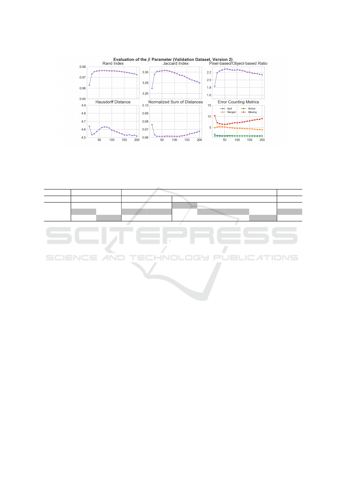
Figure 2: Average results of version 2 on the validation dataset for Rand and Jaccard Index, Hausdorff Distance, Normalized
Sum Of Distances, Error Counting Metrics and the ratio between pixel- and object-based metrics for β values from 10 to 200.
Table 1: Results of pipeline version 1 and 2 (β=50) and the CellProfiler pipeline on test dataset. Results are the average
values of the Rand and Jaccard Index, Hausdorff Distance, Normalized Sum Of Distances and Error Counting Metrics (Split,
Merged, Added, Missing) as well as the ratio between pixel- and object-based metrics. Best results are marked in gray.
Pixel-based Object-based
Version RI JI HD NSD Split Merged Added Missing Ratio
1 0.9778 4.1928 4.7973 0.0684 0.7000 5.7600 1.4400 6.3000 2.7120
2 0.9788 4.1947 4.6611 0.0645 1.1000 5.3200 1.4000 5.7400 2.8293
CP 0.9701 4.2115 5.1847 0.0946 1.3400 6.8600 5.0200 4.3800 2.2648
parameter could be done automatically by determin-
ing the maximum of the ratio of pixel- to object-based
metrics. This leads to β = 50 for the dataset used. As
can be seen in table 1, the fixed value turns out to be
a suitable setting for the whole test set on the aver-
age. The values for pixel-based metrics differ only
slightly between the compared versions. In contrast,
the object-based metrics clearly indicate that our pro-
posed pipeline achieves superior performance. This is
also confirmed by the overall higher ratio values. Be-
fore using the segmentation pipeline on a new dataset,
especially with images from other modalities, it will
still be necessary to redefine the β value and poten-
tially adjust the preprocessing.
Also other segmentation pipelines were evaluated
on the BBBC039v1 dataset. Compared to deep learn-
ing methods as presented in Caicedo et al. (2018),
the proposed pipeline perform a little worse in terms
of Merged- and Split-error. Missing-errors are again
lower for our pipeline, but this may also be due to
the different calculation of the JI. Liu et al. (2021)
have also evaluated several deep learning methods us-
ing this dataset. Their evaluation metrics differ from
those in this paper, which makes a direct comparison
difficult.
The results of the random-walk algorithm signif-
icantly depend on the seed placement. For optimal
segmentation, one seed must be set at a suitable lo-
cation for each nucleus. Because expert knowledge
to set seeds involves a great deal of effort we pro-
posed an automatic approach, described in section
3. Approaches for automatic seed determination for
random walk have already been explored for specific
problems, such as tumor or liver segmentation, and
different modalities (e.g. 3D CT, 3D MRI) (Wang
et al., 2019). Intensity values of pixels are often used
for seed determination.
We use intensity values to distinguish nuclei from
the background in fluorescence microscopy images.
Due to a combination of thresholds and local max-
ima, appropriate seeds can be selected. By using the
distance transformation, additional information about
the shape of the objects is included. From the results
shown in table 1 it can be concluded that the proposed
seed detection methods are suitable for this setting.
Since the two proposed versions differ only in the use
of a distance transformation before seed detection, it
can be concluded that such a transformation improves
seed detection in cell nuclei images. Yet, it should be
noted that it causes more Split-errors. This type of
error occurs more often for nuclei that have an elon-
gated shape and are notched in the middle. For the
present dataset, this effect occurs only sporadically.
When using the pipeline with other data or methods,
the detection method should then be selected accord-
ing to the prevailing nuclei shapes.
For some images in the dataset segmentation is
particularly challenging. One example are images
BIOIMAGING 2022 - 9th International Conference on Bioimaging
108

Ground truth version 1 version 2 CellProfiler
Figure 3: Example results for version 1, version 2 and CP version using images of the BBBC039v1 dataset compared with
the ground truth. Cropped images are shown in which the objects are randomly coloured.
that are highly noisy or show artifacts. For the former,
the ground truth for this image is empty and shows
no nuclei. Therefore results for such images are not
included in the evaluation because neither the calcu-
lation of the HD nor the NSD would be possible, as
reference objects are needed for the calculations of
both metrics. This affects two images in training set
and one image in validation set.
Due to different phenotypes, the sizes of the nuclei
can vary greatly. In order not to determine seeds for
artifacts in the image, small objects are filtered out
as described in section 3. The downside of this ap-
proach is that no seeds are determined for a large part
of the micronuclei. These nuclei are either segmented
as part of the background or merged with nuclei in
the neighborhood. The hole inside toroidal nuclei can
also be a challenge for segmentation method because
a strong intensity gradient exists between the hole and
the rest of the nucleus. Due to the random-walk algo-
rithm’s property of creating only smooth segmenta-
tions, the pipeline is robust to these morphologies as
long as only one seed is set per nuclei.
Additionally, the shapes created by touching nu-
clei can influence the segmentation. Smaller nuclei
can form structures that resemble shapes of larger nu-
clei. After a distance transformation, no adequate
number of seeds can be found because only the nuclei
that have the greatest distance to the background re-
ceive a seed, resulting in more Merged- and Missing-
errors. If the contrast is very low, even cutting out the
transformation only improves the results slightly. The
same effect on ECM applies to images with strong
artifacts, which cause a strongly reduced contrast in
both bright and dark areas. In addition, the number
of Added-errors is higher because some objects are
significantly larger than in the ground truth.
The runtime of methods based on the random-
walk is known to depend on the speed with which
the linear system of equations can be solved (Wang
et al., 2019). Our background seed detection can save
runtime because many background pixels are already
labeled. Since the number of these pixels varies, the
variance of the running time per image remains high.
This yields in a runtime of around 3 minutes (64 Bit
Windows, i5-10400 2.90GHz, 16GB RAM) for the
whole test dataset.
Throughout the pipeline, different values (e.g.
maximum object size and minimum distance of seeds)
must be set. These values should be selected accord-
ing to the available metadata. Since different magni-
fications can be used for microscopy images, a calcu-
lation, e.g. based on the resolution, is not useful.
8 CONCLUSION
In the context of this paper, two versions of a pipeline
were developed which use the random-walk algo-
rithm to segment nuclei. The versions differ in their
seed detection, as the second version uses a distance
transformation. We propose a way of determining the
free parameter of the random walk automatically by
using the ratio of the evaluation metrics.
For a benchmark dataset with fluorescence mi-
croscopy images, both versions achieve good results
with respect to different evaluation metrics. These re-
sults and the comparison with the CP pipeline show
that the developed pipeline is suitable for segment-
ing fluorescence microscopy images of nuclei. Es-
pecially for object-based evaluation metrics, the two
developed versions consistently reliably achieve good
values. The pipeline is robust against different mor-
phologies of the cell nuclei. However, micronuclei
are often missing in the segmentation results because
corresponding seeds are not generated.
Many typical challenges of a medical context are
included in the dataset used. This allows an evalua-
tion of the pipeline in terms of its use in such a setting.
The heterogeneity of the image data poses a challenge
Random-walk Segmentation of Nuclei in Fluorescence Microscopic Images with Automatic Seed Detection
109

for segmentation algorithms and seed detection. The
latter has a great influence on the quality of the seg-
mentation. The use of local maxima as seeds and the
developed method to determine a background seed is
suitable for the present dataset. The results can be
further improved by a preceding distance transforma-
tion, but results in more Split-errors. However, fur-
ther evaluations on other data sets are needed to make
a more general statement on performance.
Following aspects can also be content of further
research: An extension of the range of intensity val-
ues when handling the images to use the full 16 bits of
the TIFF images instead of 8 bits. Improving the run-
time by using further preprocessing or other solvers
for the system of equations. It is also interesting to
explore how the pipeline can be used for 3D data.
The results of this paper can further serve as a ba-
sis for an integration of the random-walk algorithm
in more sophisticated pipelines based on deep learn-
ing (e.g. as post-processing). We are planning fur-
ther evaluation and testing of this kind of integration.
In addition, the developed pipeline is suitable to pro-
vide reference benchmark results for the evaluation of
other segmentation methods.
ACKNOWLEDGMENTS
This work has been supported by the European Union
and the federal state of North-Rhine-Westphalia
(EFRE-0801303).
REFERENCES
Abdolhoseini, M., Kluge, M. G., Walker, F. R., and John-
son, S. J. (2019). Segmentation of heavily clustered
nuclei from histopathological images. Scientific re-
ports, 9(1):4551.
Caicedo, J. C., Roth, J., Goodman, A., Becker, T., Karhohs,
K. W., Broisin, M., Csaba, M., McQuin, C., Singh, S.,
Theis, F., and Carpenter, A. E. (2019). Evaluation of
deep learning strategies for nucleus segmentation in
fluorescence images. Cytometry, (95):925–965.
Coelho, L. P., Shariff, A., and Murphy, R. F. (2009).
Nuclear segmentation in microscope cell images:
A hand-segmented dataset and comparison of algo-
rithms. Proceedings. IEEE International Symposium
on Biomedical Imaging, 5193098:518–521.
Esfahani, K., Roudaia, L., Buhlaiga, N., Del Rincon, S. V.,
Papneja, N., and Miller, W. H. (2020). A review of
cancer immunotherapy: from the past, to the present,
to the future. Current oncology (Toronto, Ont.),
27(Suppl 2):87–97.
Grady, L. (2006). Random walks for image segmentation.
IEEE transactions on pattern analysis and machine
intelligence, 28(11):1768–1783.
Jaccard, P. (1901).
´
Etude comparative de la distribution flo-
rale dans une portion des alpes et du jura. Bulletin
de la Soci
´
et
´
e Vaudoise des Sciences Naturelles, pages
547–579.
Kowal, M.,
˙
Zejmo, M., Skobel, M., Korbicz, J., and Mon-
czak, R. (2020). Cell nuclei segmentation in cytolog-
ical images using convolutional neural network and
seeded watershed algorithm. Journal of Digital Imag-
ing, 33(1):231–242.
Li, C. H. and Lee, C. K. (1993). Minimum cross entropy
thresholding. Pattern Recognition, 26(4):617–625.
Liu, D., Zhang, D., Song, Y., Huang, H., and Cai, W.
(2021). Panoptic feature fusion net: A novel instance
segmentation paradigm for biomedical and biologi-
cal images. IEEE Transactions on Image Processing,
30:2045–2059.
Ljosa, V., Sokolnicki, K. L., and Carpenter, A. E. (2012).
Annotated high-throughput microscopy image sets for
validation. Nature Methods, 9(7):637.
Niforou, K. M., Anagnostopoulos, A. K., Vougas, K., Kit-
tas, C., Gorgoulis, V. G., and Tsangaris, G. T. (2008).
The proteome profile of the human osteosarcoma u2os
cell line. Cancer genomics & proteomics, 5(1):63–78.
Rand, W. M. (1971). Objective criteria for the evaluation of
clustering methods. Journal of the American Statisti-
cal Association, 66(336):846–850.
Sonka, M., Hlavac, V., and Boyle, R. (2015). Image
Processing, Analysis, and Machine Vision. Cengage
Learning, Stamford, Conn., 4. ed., internat. student ed.
edition.
Wang, P., He, Z., and Huang, S. (2017). An improved ran-
dom walk algorithm for interactive image segmenta-
tion. In Liu, D., Xie, S., Li, Y., Zhao, D., and El-
Alfy, E.-S. M., editors, Neural information process-
ing: 24th International Conference, ICONIP 2017,
Guangzhou, China, November 14-18, 2017 : proceed-
ings, Lecture Notes in Computer Science, pages 151–
159, Cham. Springer.
Wang, Z., Guo, L., Wang, S., Chen, L., and Wang, H.
(2019). Review of random walk in image processing.
Archives of Computational Methods in Engineering,
26(1):17–34.
Wirth, F., Brinkmann, E.-M., and Brinker, K. (2020). On
benchmarking cell nuclei segmentation algorithms for
fluorescence microscopy. In Proceedings of the 13th
International Joint Conference on Biomedical Engi-
neering Systems and Technologies - BIOIMAGING,
pages 164–171.
World Health Organization (2021). Can-
cer. https://www.who.int/news-room/fact-
sheets/detail/cancer (accessed 08.04.2021).
Zaki, G., Gudla, P. R., Lee, K., Kim, J., Ozbun, L., Shachar,
S., Gadkari, M., Sun, J., Fraser, I. D. C., Franco,
L. M., Misteli, T., and Pegoraro, G. (2020). A deep
learning pipeline for nucleus segmentation. Cytome-
try Part A, 97(12):1248–1264.
BIOIMAGING 2022 - 9th International Conference on Bioimaging
110
