3D Detection of Vehicles from 2D Images in Trafﬁc Surveillance

M. H. Zwemer

1,2 a

, D. Scholte

1,2

, R. G. J. Wijnhoven

2 b

and P. H. N. de With

1 c

Department of Electrical Engineering, Eindhoven University, Eindhoven, The Netherlands

ViNotion BV, Eindhoven, The Netherlands

Keywords:

3D Object Detection, Trafﬁc Surveillance, Vehicle Detection.

Abstract:

Trafﬁc surveillance systems use monocular cameras and automatic visual algorithms to locate and observe

trafﬁc movement. Object detection results in 2D object boxes around vehicles, which relate to inaccurate

real-world locations. In this paper, we employ the existing KM3D CNN-based 3D detection model, which

directly estimates 3D boxes around vehicles in the camera image. However, the KM3D model has only been

applied earlier in autonomous driving use cases with different camera viewpoints. However, 3D annotation

datasets are not available for trafﬁc surveillance, requiring the construction of a new dataset for training the 3D

detector. We propose and validate four different annotation conﬁgurations that generate 3D box annotations

using only camera calibration, scene information (static vanishing points) and existing 2D annotations. Our

novel Simple box method does not require segmentation of vehicles and provides a more simple 3D box

construction, which assumes a ﬁxed predeﬁned vehicle width. The Simple box pipeline provides the best 3D

object detection results, resulting in 51.9% AP3D using KM3D trained on this data. The 3D object detector

can estimate an accurate 3D box up to a distance of 125 meters from the camera, with a median middle point

mean error of only 0.5-1.0 meter.

1 INTRODUCTION

Vehicle trafﬁc congestion is a major problem world-

wide. Trafﬁc surveillance systems can help to im-

prove trafﬁc management in the city and ensure road

and trafﬁc safety. Such trafﬁc surveillance systems

commonly use networks of monocular cameras and

employ computer vision algorithms to observe traf-

ﬁc movement. These camera systems employ object

detection and tracking to collect statistics such as the

number of vehicles per trafﬁc lane, the type of vehi-

cles and the trafﬁc ﬂow.

Typical trafﬁc analysis systems for surveillance

cameras use an object detector to localize vehicles

followed by a tracking algorithm to follow vehicles

over time. Object locations in computer vision are

typically represented by a 2D box fully capturing the

object. The bottom midpoint of the box is then used

to deﬁne the vehicle position in a single location (see

Figure 1). The ground surface of the object is thereby

represented in a single point only. Using the camera

calibration, this pixel-position point can be converted

https://orcid.org/0000-0003-0835-202X

https://orcid.org/0000-0001-8837-3976

https://orcid.org/0000-0002-7639-7716

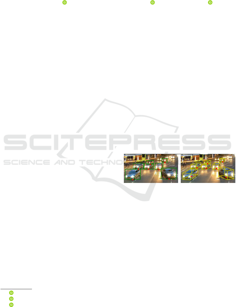
Figure 1: Localization using 2D and 3D bounding boxes.

Note the difference between the estimated ground-plane lo-

cation (red dot) for both bounding boxes.

to a real-world (GPS) location for further use in the

trafﬁc application. A more accurate detection method

would represent the object location by a 3D bounding

box such that the complete ground plane is estimated

in contrast to the current single point. The use of more

accurate 3D location estimation enables more accu-

rate measurements of vehicle speed, size and inter-

vehicle distances.

In this paper, we propose to use a 3D bounding-

box detector on monocular ﬁxed-camera images. We

assume that the cameras are fully calibrated such

that the camera locations can be converted to 3D-

world positions. Detectors that directly estimate

3D boxes (Li, 2020) from 2D images, require 3D-

labeled training datasets, which are not available

for our trafﬁc surveillance application. Available

trafﬁc surveillance datasets lack camera calibrations

Zwemer, M., Scholte, D., Wijnhoven, R. and de With, P.

3D Detection of Vehicles from 2D Images in Trafﬁc Surveillance.

DOI: 10.5220/0010783600003124

In Proceedings of the 17th International Joint Conference on Computer Vision, Imaging and Computer Graphics Theory and Applications (VISIGRAPP 2022) - Volume 5: VISAPP, pages

97-106

ISBN: 978-989-758-555-5; ISSN: 2184-4321

and 3D box annotations. Such 3D annotations are

available in datasets for autonomous driving such

as KITTI (Geiger et al., 2012), but the in-car cam-

era viewpoints are different from typical road-side

surveillance viewpoints. We propose a novel anno-

tation processing chain that converts existing 2D box

labels to 3D boxes using labeled scene information.

This labeled scene information is derived from 3D

geometry aspects of the scene, such as the vanishing

points per region and the estimated vanishing points

per vehicle depending on the vehicle orientation. The

use of vanishing points combined with camera cali-

bration parameters enables to derive 3D boxes captur-

ing the car geometry in a realistic setting. For validat-

ing the concept, the existing KM3D (Li, 2020) CNN

object detector is evaluated on our automatically an-

notated trafﬁc surveillance dataset to investigate the

effect of different processing conﬁgurations, in order

to optimize the system into a ﬁnal pipeline.

The remainder of this paper is structured as fol-

lows. First, a literature overview is given in Section 2.

Second, the 3D box annotation processing chain is

elaborated in Section 3. The results of the experi-

ments are presented in Section 4 where also the op-

timal pipeline is determined. Section 5 discusses the

conclusions.

2 RELATED WORK

There are two categories of 3D object detectors for

monocular camera images: (A) employing geometric

constraints and labeled scene information and (B) di-

rect estimation of the 3D box from a single 2D image.

A. Geometric Methods. In (Dubsk

a et al., 2014),

the authors propose an automatic camera calibration

from vehicles in video. This calibration and vanishing

points are then used to convert vehicle masks obtained

by background modeling to 3D boxes. They assume

a single set of vanishing points per scene, as the road

surface in the scenes are straight and the camera posi-

tion is stationary. The authors of (Sochor et al., 2018)

improve vehicle classiﬁcation using information from

3D boxes. Because their method works on static 2D

images and motion information is absent to estimate

the object orientation, they propose a CNN to esti-

mate the orientation of the vehicle. With the vehicle

orientation and camera calibration the 3D box is esti-

mated based on work of (Dubsk

a et al., 2014). In our

case, we adopt the 3D box generation from Dubsk

a et

al., but instead of using the single road direction (per

scene) for each vehicle, we calculate the orientation

for each vehicle independently. This enables to ex-

tend the single-road case to scenes with multiple vehi-

cle orientations, such as road crossings, roundabouts

and curved roads.

B. Direct Estimation by Object Detection. Early

work uses a generic 3D vehicle model that is pro-

jected to 2D given the vehicle orientation and cam-

era calibration and then matched to the image. The

authors of (Sullivan et al., 1997) use an 3D wire-

frame model (mesh) and match it on detected edges in

the image and Nilsson and Arn

o (Nilsson and Ard

2014) use foreground/background segmentation. Ve-

hicle matching is sensitive to the estimated vehicle

position, the scale/size of the model, and the vehicle

type (stationwagon vs. hatchback). Histogram of Ori-

ented Gradients (HOG) (Dalal and Triggs, 2005) gen-

eralizes the viewpoint speciﬁc wire-frame model to a

single detection model. Wijnhoven et al. (Wijnhoven

and de With, 2011) divide this single detection model

into separate viewpoint-dependent models.

State-of-the-art CNN detectors generalize into a

multi-layer detection system. Here, the vehicle and

its 3D pose are estimated directly from the 2D im-

age. Most methods use two separate CNNs or ad-

ditional layers. Depth information is used as an ad-

ditional input to segment the vehicles in the 2D im-

age in (Brazil and Liu, 2019; Ding et al., 2020; Chen

et al., 2016; Cai et al., 2020). Although the depth

is estimated from the same 2D images, it requires an

additional depth-generation algorithm. Mousavian et

al. (Mousavian et al., 2017) use an existing 2D CNN

detector and add a second CNN to estimate the ob-

ject orientation and dimensions. The 3D box is then

estimated as the best ﬁt in the 2D box, given the ori-

entation and dimensions. RTM3D (Li et al., 2020)

and KM3D (Li, 2020) estimate 3D boxes from the 2D

image directly into a single CNN. They utilize Cen-

terNet with a stacked hourglass architecture to ﬁnd

8 key points and the object center, to deﬁne the 3D

box. Whereas RTM3D utilizes the 2D/3D geometric

relationship to recover the dimension, location, and

orientation in 3D space, KM3D estimates these values

directly, which is faster and can be jointly optimized.

We adopt the KM3D model as the 3D box detector

because it is fast and can be trained end-to-end on 2D

images only.

3 SEMI-AUTOMATIC 3D

DATASET GENERATION

This section presents several techniques to semi-

automatically estimate 3D boxes from scene knowl-

edge and existing 2D annotated datasets for trafﬁc

surveillance. Estimating a 3D box in an image is car-

ried out in the following four steps (see Figure 2).

VISAPP 2022 - 17th International Conference on Computer Vision Theory and Applications

Dataset

Generation of

3D Dataset

Dataset

2D & 3D

3D Object

Detector

Training

Camera Images

3D Object

Detection

Live Operation:

3D Object

Detection

3D Object

Detector

Scene Information

Camera Calibration

2D Localization

Segmentation

Orientation

Estimation

3D Box

Generation

Oﬄine training and evalua�on:

Evaluation

3D Detec�on

Results

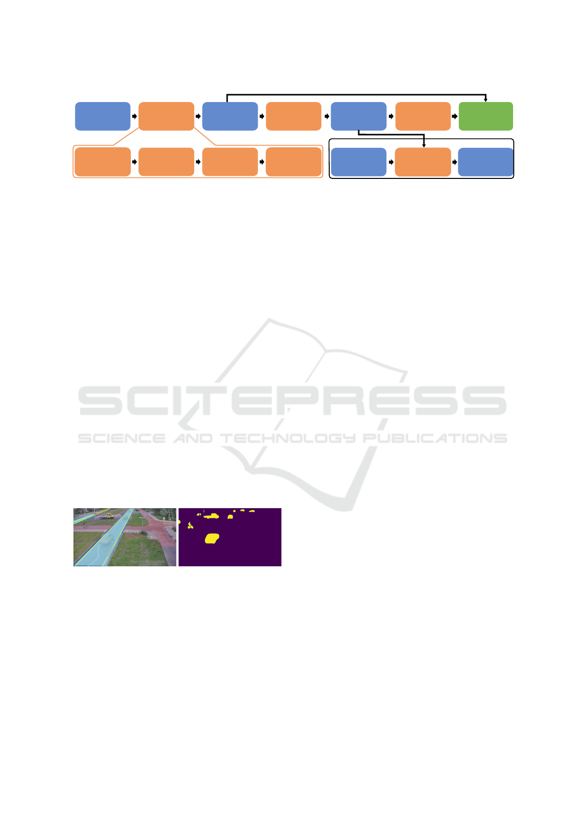
Figure 2: System overview of automatic 3D annotation of 2D images and training the 3D object detector, using inference with

live camera images.

First, a camera calibration and scene information is

created for each camera scene. Second, the 2D loca-

tion and segmentation for each vehicle is determined.

Third, the orientation of each vehicle is estimated, and

ﬁnally the 3D box is constructed. Each step is now

explained individually.

A. Prior Knowledge. The ﬁrst step is to gather scene

information from an image set and create a corre-

sponding camera calibration. Since datasets often

contain many images from the same scene, this prior

knowledge has to be generated often only once for

each unique scene, resulting in limited manual effort.

The camera calibration involves estimation of all

internal and external camera parameters to form a

camera projection matrix (Brouwers et al., 2016).

This matrix describes the mapping of a pinhole cam-

era model from 3D points in the world to 2D image

coordinates and vice versa.

The scene information consists of annotated van-

ishing points for each straight road section. The yel-

low lines in the example of Figure 3a show the lines

from each straight road section (blue area), which will

converge to the corresponding vanishing point (out-

side the image). The vanishing points are used in our

orientation estimation and 3D box-generation steps.

(a) Annotated scene. (b) Segmentation map.

Figure 3: Example scene with conﬁgured horizon lines and

2D annotated bounding-boxes (a). Blue areas show the

straight road segments, yellow lines are used to ﬁnd the

vanishing points (partially blurred for privacy reasons). The

image in (b) shows the corresponding segmentation map of

the scene.

B. Segmentation and 2D Box Locations. Object

segmentation for each vehicle is required for some

of the techniques for orientation estimation and 3D

box-generation steps. Although any algorithm that

produces a segmentation mask can be used, we em-

ploy the existing Mask-RCNN object detector with

instance segmentation (He et al., 2017) for its efﬁ-

ciency. Figure 3b show an example segmentation

map. The 2D box detections are matched with the

2D box annotations based on an Jaccard overlap (IoU)

threshold. If sufﬁcient overlap is found, the segmen-

tation is matched to our ground-truth annotation. If a

ground-truth object is not matched with a segmenta-

tion, it is removed from the training set. Detections

not matching ground-truth are ignored.

3.1 Orientation Estimation

In this subsection, the goal is to estimate the orienta-

tion of the object. The input is the scene information

(static vanishing points), camera calibration and the

2D box, while in some techniques also an object seg-

mentation is used. For each object, the output is an

orientation (angles) in the real-world domain.

The orientation estimation of all vehicles within

a straight road section is based upon the direction of

this straight section because we assume all vehicles

driving in the correct direction and orientation with

respect to these road sections. To this end, an overlap

is calculated between each 2D object bounding-box

and all the straight road sections (see blue areas in

Figure 3a). If the overlap value exceeds a threshold,

the orientation of the vehicle is parallel with the di-

rection of the considered road section (see Figure 4b).

If an object is not in a straight road section, we ap-

ply one of the techniques explained in the following

paragraphs. The techniques discussed are based on

Principal Component Analysis (PCA), PCA with ray

casting technique, and an Optical ﬂow-based method.

A. Principal Component Analysis (PCA). PCA is

applied to the collection of foreground points in the

segmentation mask. The ﬁrst principal component

corresponds to our orientation estimation which cor-

responds to the inertia axis of the segmentation mask.

Figure 4c illustrates an estimated orientation. If mul-

tiple sides of the vehicle are observed (e.g. front, top

and side of the vehicle in Figure 4c), the inertia axis of

the segmentation will be based on several sides of the

vehicle. This introduces an offset in the orientation

3D Detection of Vehicles from 2D Images in Trafﬁc Surveillance

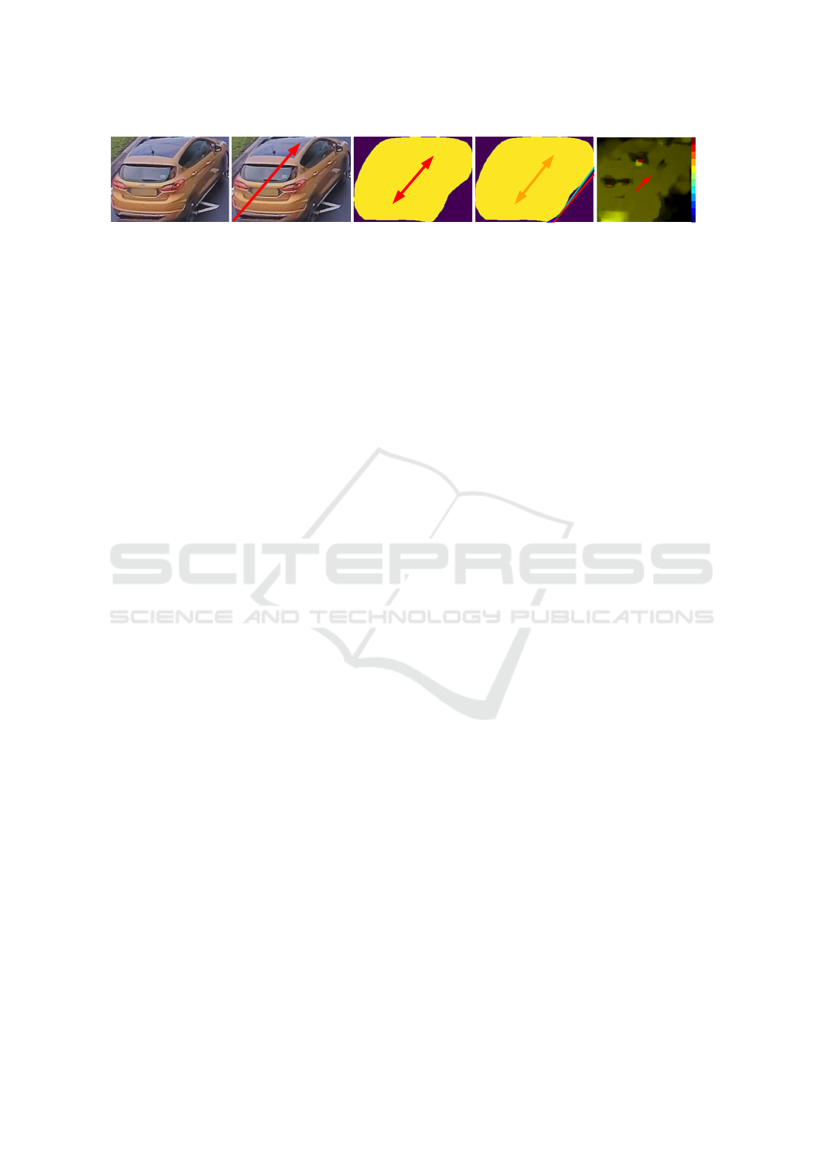
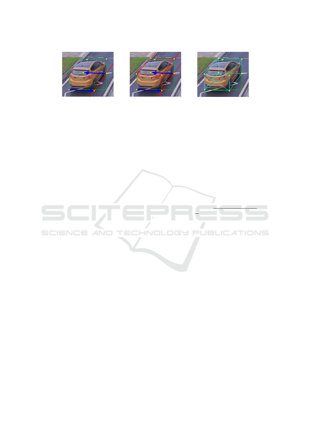
(a) Image crop. (b) Prior knowledge. (c) PCA. (d) Ray-Casting.

180

-90

-180

(e) Optical Flow.

Figure 4: Four methods (in (b)-(e)) of estimating orientation for the annotation shown in (a).

estimation. This offset depends on the orientation of

the vehicle, the tilt of the camera, and the location in

the image (e.g. far ﬁeld).

B. PCA with Ray-casting. This method is similar

to the previous implementation using PCA analysis,

but extends this method by additional post-processing

using a ray-casting algorithm. This ray-casting algo-

rithm operates in the following two steps.

First, a line with the same orientation as the ori-

entation from the above PCA is ﬁtted to the bottom

contour of the segmentation mask (when tilted right

(left), this is at the bottom-right (left) corner). This

line is shown by the red line in Figure 4d. The point

where this line intersects the segmentation contour is

the starting point of the ray-casting algorithm.

Second, a ray-casting algorithm is applied to de-

termine the edges of the contour as observed from the

intersection point (see the green dot in Figure 4d).

The ray-casting algorithm searches for a line from

the intersection point that intersects the segmenta-

tion contour at another point by evaluating multiple

lines with small orientation changes. These orienta-

tion changes are carried out in two directions, clock-

wise and counter-clockwise. The two lines resulting

from ray-casting are depicted in the bottom-right cor-

ner with dark blue and cyan lines in Figure 4d. The

orientation of the two resulting lines are compared to

the original estimated direction of the principal com-

ponents. If any of these two is close in orientation to

the starting orientation, the minimum change in ori-

entation is taken, otherwise the ray-casting-based ori-

entation is neglected and the starting orientation is in-

evitably used (ray-casting did not work).

C. Optical Flow. The last orientation estimation

method is based upon Optical ﬂow. The Optical ﬂow

algorithm measures the apparent motion of objects in

images caused by displacement of the object or move-

ment of the camera between two frames. The result

is an 2D vector ﬁeld, where each vector shows the

displacement of movement of points between the ﬁrst

and the second frame. The optical ﬂow algorithm is

based on Farneb

ack’s algorithm (Farneb

ack, 2003).

To compute the orientation for all vehicles, we

ﬁrst apply a threshold on the magnitude of the optical

ﬂow to only select pixels with sufﬁcient movement.

Next, the 2D box of each object is used to select the

ﬂow vectors that correspond to each object. The ori-

entation is then estimated as the median of the orienta-

tions of the Optical ﬂow vectors. An example of Opti-

cal ﬂow-based orientation estimation is visualized in

Figure 4e, where the background colors indicate the

motion directions of points.

3.2 3D Box Generation

The outputs of the prior knowledge, segmentation and

orientation estimation steps are the input for the con-

struction of the actual 3D boxes. Note that the meth-

ods for creating the 3D boxes in this section are only

used to create annotations to train the actual detec-

tion model. The ﬁnal detection for live operation di-

rectly estimates the 3D box using the KM3D detector

(see Figure 2). This section describes two methods

for generating 3D box annotations. The ﬁrst method

is dependent on a correct segmentation map of each

object in the scene and is called ‘Segmentation ﬁt-

ting’, while the second method ‘Simple Box’ relies

on prior information only and does not require seg-

mentation of vehicles. Note that both these methods

rely on an estimated orientation, provided by one of

the methods described in Section 3.1. On straight road

sections this estimation is based on prior knowledge.

For curved roads an estimation based on PCA, PCA

with ray-casting, or Optical ﬂow is created. Hence,

although the estimated orientation differs when a ve-

hicle is not on a straight road section, the 3D box gen-

eration methods are similar.

A. Segmentation Fitting. The generation of 3D

boxes based on a segmentation uses the box-ﬁtting

algorithm of (Dubsk

a et al., 2014), where a 3D box

is constructed using three vanishing points. The ﬁrst

vanishing point is located at the crossing of the hori-

zon line and the line in the direction of the estimated

vehicle orientation. The second point is the crossing

of the horizon line with the line orthogonal to the ve-

hicle orientation. This orientation is estimated in the

real-world domain using the camera-projection ma-

trix. The third point is the vertical vanishing point of

the scene, which results from camera calibration.

VISAPP 2022 - 17th International Conference on Computer Vision Theory and Applications

100

(a) Fitted vanishing lines.

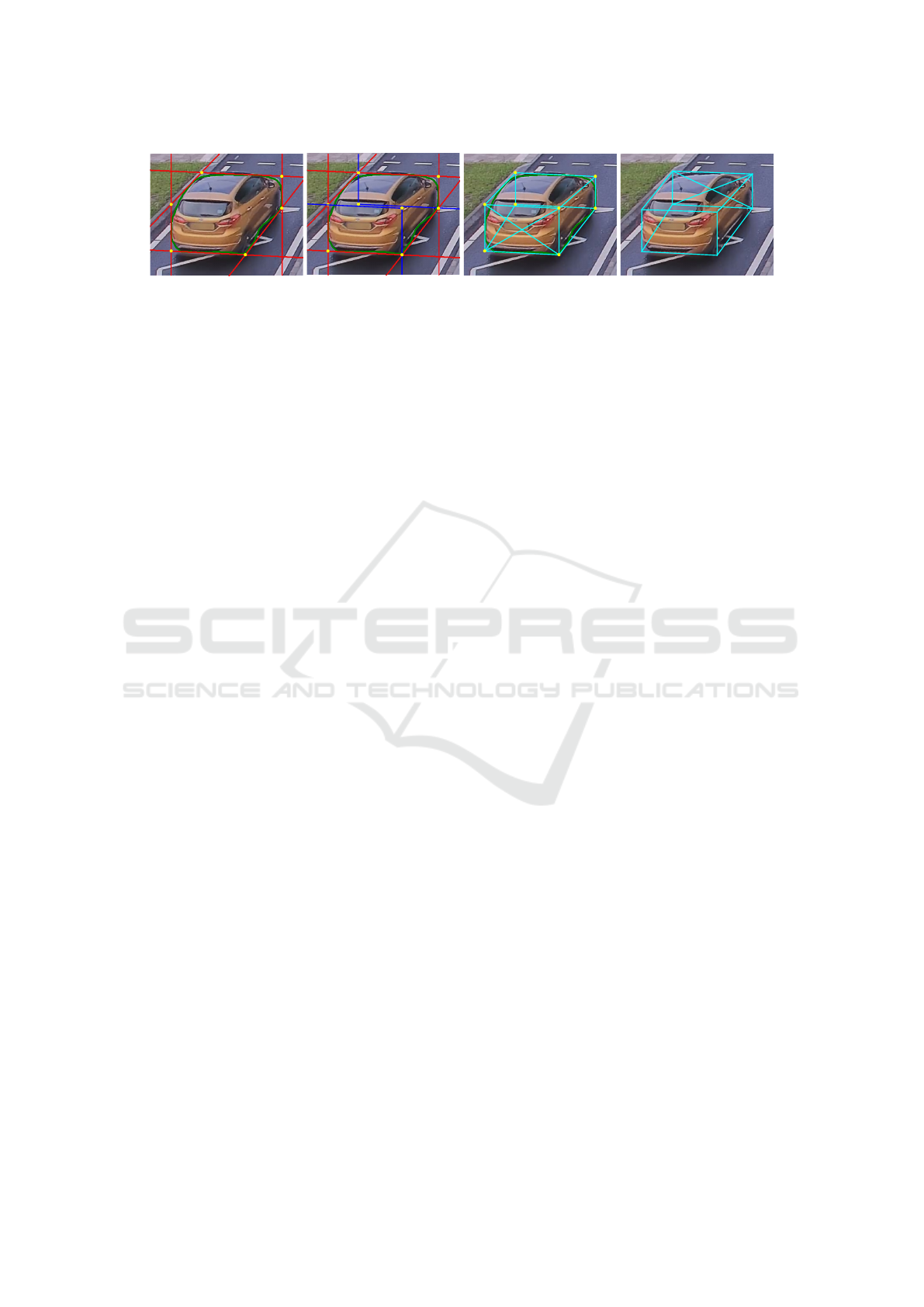
(b) Remaining points. (c) Resulting 3D box. (d) Average height 3D box.

Figure 5: Segmentation ﬁtting as the work of Dubsk

a et al.where the vanishing lines (red) are ﬁt to the contour (green). The

intersections provide corner-points (yellow) for the 3D box. The blue lines are the remaining vanishing lines used to ﬁnd the

last corner-points.

The algorithm is now as follows (based

on (Dubsk

a et al., 2014)). First, two lines are

drawn originating at each of the three vanishing

points along the sides of the contour, shown as the

six red lines in Figure 5a. At the intersections of

the lines, six corner-points of the 3D box are found,

denoted by the numbered yellow dots (1-6). The last

two corner points (7,8) are found as the intersection

of lines from corner points 2, 3, 5 and 6 towards

the vanishing points (denoted by the blue lines in

Figure 5b). The height of the different points of the

top surface can vary between corner points because

they are estimated individually. However, we assume

the roof of a vehicle to be parallel to the ground

surface and therefore use the average height of these

roof points in the ﬁnal 3D box, as shown in Figure 5d.

B. Simple Box. Instead of using a segmentation mask

for each vehicle, we propose a novel method to es-

timate a 3D box based on statistical vehicle dimen-

sions. The method requires a 2D bounding box, cam-

era calibration and the vehicle orientation, to convert

this information to a 3D box. We assume a ﬁxed ve-

hicle width and determine length and height dynami-

cally from the 2D box ﬁt. Furthermore, the three van-

ishing points are deﬁned in an identical way as in the

segmentation ﬁtting method. The 3D box generation

is carried out by the following steps.

First, we deﬁne one of the two bottom corners of

the annotated 2D box as the starting point, depending

on the estimated orientation (left- or right-facing car).

The second point is located at the end of a line seg-

ment from the ﬁrst point towards the second vanish-

ing point (orthogonal to the vehicle orientation) with

the statistical vehicle width as its length. This is de-

picted by the blue line and the points 1 and 2 in Fig-

ure 6a. The back-corner point (3) is found by deﬁn-

ing the orientation line along the length of the car at

the ground plane that crosses the 2D box, resulting

in point (3). The last ground-plane point (4) is com-

puted from the third point, by drawing a line segment

with ﬁxed length (statistical vehicle width) towards

the second vanishing point. The corner-point of the

2D box (point 5) is used as the top of the 3D box.

The vehicle height is deﬁned as the distance between

points 5 and 3 (Figure 6a). The remaining points of

the top of the 3D box can be constructed from point 5

(using the vehicle width/length), or from the ground-

plane points (using the height) (see Figure 6b). The

ﬁnal obtained 3D box is depicted in Figure 6c.

We have found that the vehicle height is often es-

timated too low, caused by small variations in the 2D

box locations and the orientation estimations. The es-

timated height is pragmatically adjusted if it is below

a threshold T

height

, by slightly modifying the orienta-

tion. The orientation estimation is updated with one

degree in a direction such that the estimated height

becomes closer to the average vehicle height. The

adapted direction depends on the orientation of the

vehicle. The threshold T

height

is deﬁned as the statis-

tical average vehicle height H

avg

minus the H

variation

value. This process of updating the orientation is re-

peated until the estimated vehicle height exceeds the

threshold. The selected threshold values are discussed

in Section 4(A).

4 EXPERIMENTS

The 3D box generation processing is evaluated with

two different approaches. First, we evaluate a direct

approach where the output of the annotation process

(without the 3D detector) is considered. Second, we

train and evaluate the performance of the 3D object

detector (KM3D (Li, 2020)) based on the output of

the box generation. In two additional experiments

with the KM3D detector, a cross-validation between

our dataset and the KITTI dataset is presented and an

unsupervised approach of the generation pipeline is

evaluated.

A. Conﬁguration. All experiments are carried out

on 4 different processing pipeline conﬁgurations. The

ﬁrst three conﬁgurations use a segmentation mask as

input for the ‘segmentation ﬁtting’ technique to esti-

mate the 3D box. The orientation estimation in each

3D Detection of Vehicles from 2D Images in Trafﬁc Surveillance

101

(a) Estimated ground-

surface points based on

vehicle width.

(b) The remaining roof

points estimated based on

vanishing lines.

Figure 6: Simple Box construction method for corner-points (yellow) of the 3D box with the assumption that a car has an

width of 1.75m (blue arrows). The other 3D corner-points are calculated through the estimated vanishing lines (red and cyan)

and their intersections.

of these three pipelines is carried out with PCA, PCA

+ ray-casting or optical ﬂow. The fourth pipeline is

based on the Simple box 3D box estimation tech-

nique, and uses Optical ﬂow-based orientation esti-

mation, such that it does not depend on an object

segmentation map. The Farneb

ack (Farneb

ack, 2003)

Optical-ﬂow algorithm is computed on a pyramid of 3

layers, where each layer is a factor of two smaller than

the previous one. The averaging window size is 15

pixels. In all experiments using a segmentation mask,

Mask-RCNN (pre-trained on the COCO dataset (Lin

et al., 2015)) is used to predict 2D boxes and the cor-

responding object segmentation. The Mask-RCNN

segmentation masks have proven to be accurate for

vehicles in surveillance scenarios. The detection

threshold is set to 0.75 and a minimum IoU thresh-

old of 0.5 is applied to match between detections and

ground-truth boxes. For the Simple box method, the

vehicle width is set to 1.75 meters and the average

height H

avg

= 1.5 meters. We have empirically de-

termined a maximum offset of H

variation

= 0.25 me-

ters with respect to the statistical average height H

avg

resulting in T

height

= 1.3 m. For training the KM3D

model, we have used the parameters, data prepara-

tion and augmentation process from the original im-

plementation (Li, 2020). We train for 50 epochs using

learning rate 5 × 10

−5

and a batch size of 16.

B. Trafﬁc Surveillance Dataset. Our experiments

are carried out on a proprietary trafﬁc surveillance

dataset annotated with 2D boxes. This dataset con-

tains 25 different surveillance scenes of different traf-

ﬁc situations like roundabouts, straight road sections

and various crossings. The dataset is split in 20k train-

ing images and 5k validation images, with 60k and

15k annotations, respectively. The ground-truth test

set used for evaluation consists of 102 images with

444 3D boxes which are manually annotated. This

set contains 8 different surveillance scenes, which are

outside the training and validation sets. In all ex-

periments except the cross-validation experiment, we

combine the train dataset from KITTI (Geiger et al.,

2012) with the train part of our dataset to increase the

amount of data.

C. Evaluation Metrics. In our experiments, we mea-

sure the average precision 3D IoU (AP3D) and av-

erage orientation similarity (AOS), as deﬁned by the

KITTI dataset (Geiger et al., 2012), with two differ-

ent IoU thresholds of 50% and 70%. Next to these

existing metrics, we introduce the Middle point Mean

Error (MME) of the ground surface. This MME is

deﬁned as:

MME =

N−1

∑

i=0

( ˆx

− x

)

+ ( ˆy

− y

)

, (1)

where N is the total number of true positive detec-

tions, ˆx and ˆy are the ground-truth x- and y-locations

of the middle-point on the ground surface in real-

world coordinates, where x and y are the estimated

x- and y-locations. This metric depicts the aver-

age location error of the center point on the ground

plane in 3D world-coordinates (ignoring the vehicle

width/height/length dimension).

4.1 Optimizing 3D Annotation Pipeline

This experiment evaluates the four different annota-

tion pipeline conﬁgurations, which create 3D annota-

tions from the existing 2D annotated datasets. To this

end, all pipelines are executed on the testing dataset,

where the 2D annotated boxes of the testing dataset

are used as input. The resulting 3D boxes generated

by the different pipelines are compared with the man-

ually annotated 3D boxes in the testing dataset.

The results of the proposed pipelines are shown

in the left part of Table 1. The Simple box pipeline

clearly results in the best detection score (IoU=0.5)

with 36.4% mAP for Hard objects, most accurate

center-point estimation (MME=0.66) and best orien-

tation estimation (AOS=93.8). Note that detection

performance for the strict IoU=0.7 evaluation is very

VISAPP 2022 - 17th International Conference on Computer Vision Theory and Applications

102

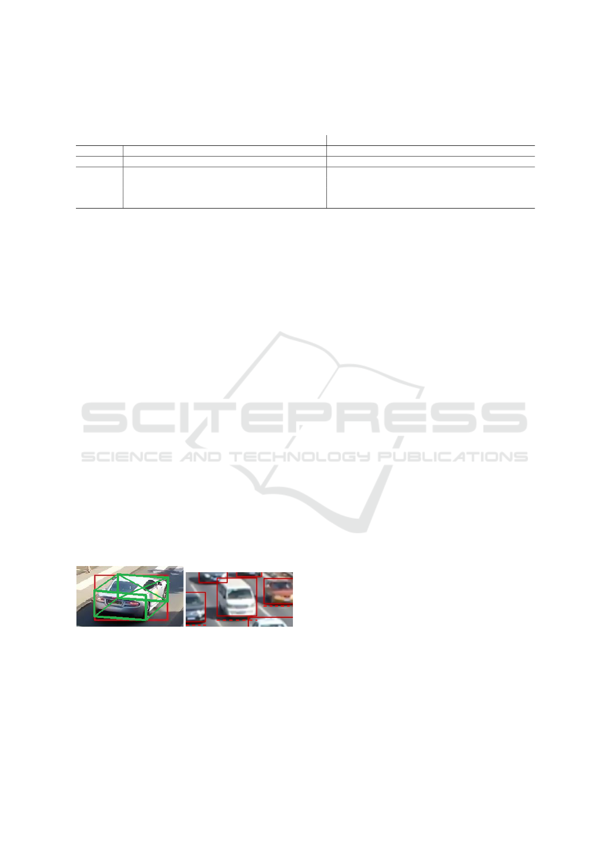
Table 1: Comparison of 3D annotation processing conﬁgurations without 3D object detector (left) and the same comparison

for the 3D annotation conﬁgurations with trained 3D detector on the data generated by the conﬁgurations (right). Detection

performance increases with the addition of the 3D detector (IoU=0.5). The Simple box-based pipeline is the best.

3D Annotation pipeline 3D Annotation pipeline + 3D detector

AP3D IoU=0.7 / IoU=0.5 MME AOS AP3D IoU=0.7 / IoU=0.5 MME AOS

Pipeline Easy Moderate Hard Easy Moderate Hard

PCA 5.9/42.1 5.7/37.6 3.3/23.3 0.80 84.7 2.8/53.5 2.9/49.8 2.5/35.9 0.66 89.2

RayCast. 6.0/41.9 5.8/31.7 3.3/22.9 0.80 84.9 3.5/53.3 3.6/48.0 2.9/34.0 0.85 89.4

Opt.Flow 7.1/52.0 6.5/39.5 3.8/24.8 0.71 90.0 4.2/62.8 5.6/51.0 3.8/42.9 0.66 89.5

Simple b. 18.9/59.7 13.1/46.7 9.9/36.4 0.66 93.8 26.2/73.4 19.9/62.9 15.6/51.9 0.70 89.6

limited, probably because of the inaccurate 3D boxes

generated by the pipeline. The practical performance

for IoU=0.5 is representative for the application of

video surveillance.

A. Orientation Estimation. PCA and ray-casting

both depend on the segmentation map. Whereas

PCA is dependent on the mass of the segmentation,

ray-casting ﬁts to the contours of the segmentation.

The ray-casting technique (84.9%) results in a mi-

nor improvement in AOS score with respect to PCA

(84.7%). Since the AOS scores of Optical ﬂow and

Simple box are higher, which both use Optical ﬂow

as methods for orientation estimation, it can be con-

cluded that Optical ﬂow outperforms the segmenta-

tion map-based methods. However, Optical ﬂow can-

not be computed when previous/next frames are not

available, then the ray-casting method can be used.

B. Segmentation Fitting. Visual inspection of the

3D generated box results of the segmentation ﬁtting-

based methods show that the main cause of errors

is the width and length estimation, as shown in Fig-

ure 7a. In this example, the length is estimated 1 me-

ter too short. These errors are caused by segmentation

maps that do not perfectly align with the actual ob-

ject contours. The segmentation maps do not consis-

tently include the headlights, wheels and other parts

of the vehicles and sometimes include vehicle shad-

ows. Although we always map the Mask-RCNN de-

tection and segmentation output to our ground-truth

(a) Segmentation ﬁtting. (b) Simple box.

Figure 7: Two examples of cases which result in wrongly

estimated 3D boxes. At the left-hand side, a segmentation

ﬁtting problem occurs because the front-right wheel point

is estimated too far to the right and does not extend beyond

the wheel in length. At the right-hand side, the Simple box

method will estimate the box too high because the 2D-box

bottom line does not touch the ground surface but aligns

with the vehicle bumper. The dashed red line depicts the

desired bottom line for the 2D-box.

2D bounding-boxes to ensure that no false detections

are used as 3D ground truth, we rely on the quality of

the generated segmentation maps from Mask-RCNN.

C. Simple Box. The Simple box pipeline results

in higher performance than the segmentation ﬁtting-

based methods (36.4% vs. 22-24% AP3D). From

these results we conclude that a 2D box annotation

and orientation information is sufﬁcient to estimate a

3D box. Visual inspection of the results show that

errors commonly originate from 2D bounding boxes

of which the bottom line is not touching the ground

plane. In such a case, the starting point for the Sim-

ple box method is too high, so that the constructed 3D

box ﬂoats in the air (see the examples in Figure 7b).

4.2 3D Annotation Pipeline + Detector

In this experiment, the KM3D detector is trained on

the 3D annotations generated by the different annota-

tion conﬁgurations. The performance of the KM3D

detector is measured on the test dataset.

The scores from the detection results are shown at

the right-hand side of Table 1. The addition of the 3D

detector results in a signiﬁcantly increased detection

performance (increase of 12-18% AP3D) for all con-

ﬁgurations with respect to the direct 3D annotation

pipeline results (left-hand side in Table 1). Visual in-

spection of the detection results for PCA, ray-casting

and Optical ﬂow shows that the estimated ground sur-

face is estimated better by the 3D detector than the

direct output of the annotation pipeline. This means

that the annotation quality of the generated 3D box

dataset is sufﬁcient to train a model that generalizes

over all the noisy input data.

Some detection results of the 3D detector trained

with annotations from Simple box are shown in Fig-

ure 8. These images visualize three limitations of the

method. First, not every vehicle is estimated on the

ground surface. Second, the orientation estimation of

vehicles that are driving in a horizontal direction are

prone to errors. Third, the height of the vehicles of-

ten seems to be estimated too low. However, more

detailed measurements for the estimated vehicle di-

mensions show that the height, length and width have

3D Detection of Vehicles from 2D Images in Trafﬁc Surveillance

103

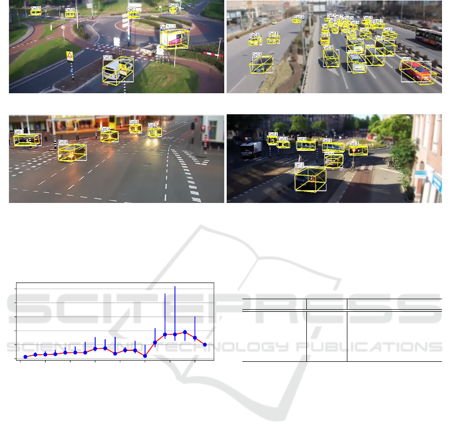
(a) Correct results in a complex scene. (b) Some faulty orientation estimations in the back.

Figure 8: Detection results of KM3D trained with the annotations generated by the SimpleBox pipeline. Partially blurred for

privacy reasons. Majority of the 3D bounding-boxes are accurately estimated.

a mean offset with respect to the ground-truth annota-

tions of 0.05, 0.02 and 0.01 meters, respectively.

Median MME per 10m

0 25 50 75 100 125 150 175

Absolute distance [m]

Figure 9: Box plot showing the median (blue dots) of the er-

ror for objects at each 10-m distance from the camera. Lines

above and under the dots represent the standard deviations

for errors estimated further away and nearby, respectively.

In a last experiment with the KM3D detector we

investigate the effect of the distance of each vehicle

to the camera on the accuracy of the 3D box esti-

mation, trained by using annotations from the Simple

box pipeline. We calculate the error in steps of 10-m

distance from the camera. The results are shown in

Figure 9. The blue dots show the median values for

each 10-m interval, the blue lines above/below rep-

resent the standard deviations of the errors of detec-

tions at larger/smaller distance. From the results, it

can be observed that accurate position estimation is

possible until about 130-m distance. The MME met-

ric becomes inaccurate from about 140-m distance,

but our test set lacks the images to validate this in

more detail. Note that the manual generation of 3D

ground-truth boxes also becomes more inaccurate at

Table 2: Cross-validation on the KITTI dataset with the

KM3D detector, based on the AP3D metric (IoU=0.5). The

3D annotations for training are generated with the Simple

box pipeline.

Train set Test set Easy Mod. Hard

KITTI KITTI 51.4 41.0 33.5

KITTI & Ours KITTI 55.3 44.7 35.2

KITTI Ours 5.2 3.87 2.3

Ours Ours 66.0 60.1 43.4

KITTI & Ours Ours 73.4 62.7 51.9

larger distance to the camera (and thus, lower resolu-

tion). Moreover, a small offset in image coordinates

far away from the camera can lead to large errors in

the real-world locations.

4.3 Cross-validation on KITTI Dataset

This experiment evaluates the baseline KM3D detec-

tor on our test set and performs a cross-validation on

the well-known KITTI dataset (Geiger et al., 2012).

Although KITTI data focuses on autonomous driving,

this will provide insight in the differences with our

application. The KM3D detector is trained indepen-

dently on KITTI, our dataset, and the combination.

Our training set annotations are generated using the

Simple box pipeline. Evaluation is carried out by in-

ference on the KITTI test set and our test set. The

results are measured by the AP3D metric.

Table 2 depicts the obtained results. The original

results on the KITTI test set are similar to the original

work (Li, 2020). Testing the KITTI-trained model on

our dataset results in poor performance because of the

VISAPP 2022 - 17th International Conference on Computer Vision Theory and Applications

104

Table 3: Detection performance when using unsupervised

Simple box pipeline (replacing 2D annotations with Mask-

RCNN output). Unsupervised performance (US) is lower

than when using the original 2D annotations.

AP3D IoU=0.5 MME

Method Easy Mod. Hard

3D annotations 59.7 46.7 36.4 0.66

3D annotations US 37.4 31.5 15.6 0.76

3D ann. + KM3D 73.4 62.9 51.9 0.70

3D ann. + KM3D US 67.3 55.8 40.7 0.65

changed viewpoints. Training on the combination of

both datasets increases the AP3D with about 3% on

the easy cases when evaluating on the KITTI dataset.

The AP3D performance on our dataset increases from

55.6% to 62.5%. Although the two datasets contain

different camera viewpoints, the detection model ef-

fectively uses this information to generalize better.

4.4 Unsupervised Approach

This experiment investigates the effect of replac-

ing the 2D box annotations with automatic detec-

tions from Mask-RCNN, thereby limiting the anno-

tation effort to scene and camera-calibration parame-

ters only. The 2D annotations which are used in the

Simple box pipeline are created using the pre-trained

Mask-RCNN detection network, instead of using the

annotated 2D boxes. We apply this modiﬁed Simple

box pipeline directly to our train and test set images

and train the KM3D detector on the output.

The results are shown in Table 3. The pipeline

with the 3D object detector has superior results over

the unsupervised conﬁguration without 3D object de-

tector. The AP3D performance gap is 20 − 25%.

The AP3D difference between the unsupervised con-

ﬁguration and the supervised conﬁguration is only

6 − 11%. Visual inspection shows that the 2D de-

tection set generated by Mask-RCNN contains many

false detections. This results in falsely annotated

3D boxes in our Simple box pipeline and causes the

KM3D detector to learn false objects. Nevertheless,

since the unsupervised pipeline is fully automatic and

requires no prior annotations, it shows opportunities

for future work.

5 CONCLUSION

We have investigated the detection of 3D bounding

boxes for objects using calibrated static monocular

cameras in trafﬁc surveillance scenes. It has been

found that it is possible to directly estimate 3D boxes

of vehicles in the 2D camera image using a 3D object

detector. We have selected the KM3D CNN-based

detection model, which has only been applied ear-

lier in autonomous driving with different viewpoints.

Although the 3D object detector can be directly ap-

plied to trafﬁc surveillance, 3D public datasets are not

available to train the 3D detection model.

Therefore, we propose a system to semi-

automatically construct 3D box annotations, by ex-

ploiting camera-calibration information and simple

scene annotations (static vanishing points). To this

end, we use existing trafﬁc surveillance datasets with

2D box annotations and propose a processing pipeline

to convert the 2D annotations to 3D boxes. The result-

ing 3D annotated dataset is used to train the KM3D

object detector. The trained 3D detector can be di-

rectly integrated in surveillance systems, as inference

only requires 2D images and camera calibration.

For optimization, we have validated four different

annotation processing conﬁgurations, each contain-

ing orientation estimation, segmentation and 3D con-

struction components. In addition to combinations

of existing components, we propose the novel Sim-

ple box method. This method does not require seg-

mentation of vehicles and provides a more simple 3D

box construction, assuming a ﬁxed predeﬁned vehicle

width. When comparing our different 3D annotation

conﬁgurations, we have found that the Simple box

pipeline provides the best object annotation results,

albeit all four conﬁgurations result in accurate orien-

tation estimation and localization. Using the 3D box

annotations from Simple box directly (without the 3D

object detector), the AP3D score is 36.4% which im-

proves to 51.9% AP3D when using KM3D trained on

this data. Similarly, we have found that the differ-

ent viewpoints from the KITTI autonomous driving

dataset actually increase performance when adding it

to our trafﬁc set.

The experimental results show that it is possible to

use a 2D dataset to generate a 3D dataset. It has been

shown that the existing KM3D object detector trained

on the generated dataset generates more accurate 3D

vehicle boxes than the vehicle annotations from the

proposed automatic 3D annotation pipeline, due to its

capacity to generalize. The resulting 3D box detec-

tions are accurate (51.9% AP3D), both in locations

and size, up to about 125 meters from the camera. The

use of unsupervised annotation using existing 2D de-

tectors can potentially increase the 3D detection per-

formance even further.

REFERENCES

Brazil, G. and Liu, X. (2019). M3d-rpn: Monocular 3d

region proposal network for object detection.

3D Detection of Vehicles from 2D Images in Trafﬁc Surveillance

105

Brouwers, G., Zwemer, M., Wijnhoven, R., and With, P.

(2016). Automatic calibration of stationary surveil-

lance cameras in the wild. In Proc. of the IEEE CVPR.

Cai, Y., Li, B., Jiao, Z., Li, H., Zeng, X., and Wang, X.

(2020). Monocular 3d object detection with decou-

pled structured polygon estimation and height-guided

depth estimation. In AAAI.

Chen, X., Kundu, K., Zhang, Z., Ma, H., Fidler, S., and

Urtasun, R. (2016). Monocular 3d object detection

for autonomous driving. In Proc. of the IEEE CVPR.

Dalal, N. and Triggs, B. (2005). Histograms of oriented

gradients for human detection. In 2005 IEEE com-

puter society conference on computer vision and pat-

tern recognition (CVPR’05), volume 1, pages 886–

893. Ieee.

Ding, M., Huo, Y., Yi, H., Wang, Z., Shi, J., Lu, Z., and

Luo, P. (2020). Learning depth-guided convolutions

for monocular 3d object detection. In Proc. of the

IEEE/CVF Conference on CVPR.

Dubsk

a, M., Herout, A., and Sochor, J. (2014). Auto-

matic camera calibration for trafﬁc understanding. In

BMVC, volume 4,6, page 8.

Farneb

ack, G. (2003). Two-frame motion estimation based

on polynomial expansion. In Scandinavian Conf. on

Image Analysis. Springer.

Geiger, A., Lenz, P., and Urtasun, R. (2012). Are we ready

for autonomous driving? the kitti vision benchmark

suite. In Conf. on CVPR.

He, K., Gkioxari, G., Doll

ar, P., and Girshick, R. (2017).

Mask r-cnn. In Proc. of the IEEE ICCV.

Li, P. (2020). Monocular 3d detection with geometric con-

straints embedding and semi-supervised training.

Li, P., Zhao, H., Liu, P., and Cao, F. (2020). Rtm3d:

Real-time monocular 3d detection from object key-

points for autonomous driving. arXiv preprint

arXiv:2001.03343.

Lin, T.-Y., Maire, M., Belongie, S., Bourdev, L., Girshick,

R., Hays, J., Perona, P., Ramanan, D., Zitnick, C. L.,

and Doll

ar, P. (2015). Microsoft coco: Common ob-

jects in context.

Mousavian, A., Anguelov, D., Flynn, J., and Kosecka, J.

(2017). 3d bounding box estimation using deep learn-

ing and geometry.

Nilsson, M. and Ard

o, H. (2014). In search of a car - uti-

lizing a 3d model with context for object detection.

In Proceedings of the 9th International Conference on

Computer Vision Theory and Applications - Volume

2: VISAPP, (VISIGRAPP 2014), pages 419–424. IN-

STICC, SciTePress.

Sochor, J.,

Spa

nhel, J., and Herout, A. (2018). Boxcars: Im-

proving ﬁne-grained recognition of vehicles using 3-d

bounding boxes in trafﬁc surveillance. IEEE transac-

tions on intelligent transportation systems.

Sullivan, G. D., Baker, K. D., Worrall, A. D., Attwood, C.,

and Remagnino, P. (1997). Model-based vehicle de-

tection and classiﬁcation using orthographic approxi-

mations. Image and vision computing, 15(8):649–654.

Wijnhoven, R. G. and de With, P. H. (2011). Unsuper-

vised sub-categorization for object detection: Find-

ing cars from a driving vehicle. In 2011 IEEE Inter-

national Conference on Computer Vision Workshops

(ICCV Workshops), pages 2077–2083. IEEE.

VISAPP 2022 - 17th International Conference on Computer Vision Theory and Applications

106