Deep Video Frame Rate Up-conversion Network using Feature-based

Progressive Residue Reﬁnement

∗

Jinglei Shi, Xiaoran Jiang and Christine Guillemot

INRIA Rennes - Bretagne Atlantique, Campus Universitaire de Beaulieu, 35042 Rennes, France

Keywords:

Video Frame Rate Up-conversion, Frame Interpolation, Progressive Residue Reﬁnement, Optical Flow

Estimation.

Abstract:

In this paper, we propose a deep learning-based network for video frame rate up-conversion (or video frame

interpolation). The proposed optical ﬂow-based pipeline employs deep features extracted to learn residue

maps for progressively reﬁning the synthesized intermediate frame. We also propose a procedure for ﬁne-

tuning the optical ﬂow estimation module using frame interpolation datasets, which does not require ground

truth optical ﬂows. This procedure is effective to obtain interpolation task-oriented optical ﬂows and can be

applied to other methods utilizing a deep optical ﬂow estimation module. Experimental results demonstrate

that our proposed network performs favorably against state-of-the-art methods both in terms of qualitative and

quantitative measures.

1 INTRODUCTION

Video frame rate plays a critical role in video quality

perception, hence in the user quality of experience in

multimedia applications. Generating high frame rate

videos from low frame rate versions has long been a

challenging problem that has attracted a lot of atten-

tion in the computer vision community. This explains

why, in recent years, a signiﬁcant effort has been ded-

icated to the problem of video temporal interpolation

for frame rate conversion. Existing video frame in-

terpolation (VFI) approaches consist of synthesizing

intermediate frames from given input frames and can

be roughly classiﬁed into three categories, i.e. op-

tical ﬂow (Liu et al., 2017; Jiang et al., 2018; Bao

et al., 2019a; Niklaus and Liu, 2018; Niklaus and

Liu, 2020) or feature ﬂow-based schemes (Gui et al.,

2020), kernel-based schemes (Niklaus et al., 2017a;

Niklaus et al., 2017b; Bao et al., 2019b) and phase-

based ones (Meyer et al., 2015; Meyer et al., 2018).

Flow-based methods estimate optical ﬂows be-

tween given frames, then interpolate or extrapolate

target frames along the motion vectors. Liu et al. (Liu

et al., 2017) proposed a Deep Voxel Flow (DVF) net-

work that consists of a ﬂow estimation module and

a trilinear interpolation layer. The network estimates

∗

This work was supported by the EU H2020 Re-

search and Innovation Programme under grant agreement

No 694122 (ERC advanced grant CLIM).

a kind of optical ﬂow and a temporal mask for tri-

linear blending the input frames. Jiang et al. (Jiang

et al., 2018) propose a double U-Net pipeline where

the ﬁrst U-Net predicts bi-directional optical ﬂows to

be further combined to approximate the intermediate

optical ﬂows. The second U-Net reﬁnes the interme-

diate optical ﬂows as well as predicts soft visibility

maps in order to warp and linearly merge the input

frames. Bao et al. (Bao et al., 2019a) exploit depth

information in the ﬂow projection procedure for bet-

ter handling occlusions. The proposed model warps

the input frames, depth maps, and contextual features

based on the optical ﬂows, and local interpolation ker-

nels are also used for synthesizing the output frames.

In (Niklaus and Liu, 2018; Niklaus and Liu, 2020),

the authors employ the state-of-the-art PWC-Net (Sun

et al., 2018) for optical ﬂow estimation. Both in-

put frames and extracted deep features are projected

and merged to obtain intermediate frames. Instead

of using classical optical ﬂow estimation techniques,

the authors in (Gui et al., 2020) propose a two-stage

frame interpolation pipeline where feature ﬂows es-

timated by a multi-ﬂow multi-attention generator are

used to warp feature maps. For methods (Bao et al.,

2019a; Niklaus and Liu, 2018; Niklaus and Liu, 2020)

that make use of an off-the-shelf optical ﬂow estima-

tion module, they both rely on a good initialization of

that module whether or not end-to-end ﬁnetuning is

conducted later. However, most optical ﬂow estima-

Shi, J., Jiang, X. and Guillemot, C.

Deep Video Frame Rate Up-conversion Network using Feature-based Progressive Residue Reﬁnement.

DOI: 10.5220/0010793900003124

In Proceedings of the 17th International Joint Conference on Computer Vision, Imaging and Computer Graphics Theory and Applications (VISIGRAPP 2022) - Volume 4: VISAPP, pages

331-339

ISBN: 978-989-758-555-5; ISSN: 2184-4321

331

tion networks are trained on synthetic datasets with

ground truth optical ﬂows, and are not fully adapted

to the frame interpolation problem. In this paper, we

propose a simple but effective ﬁnetuning procedure

that allows us to ﬁnetune the initial optical ﬂow esti-

mation module with no need for ground truth optical

ﬂows.

Unlike ﬂow-based methods, kernel-based meth-

ods (Niklaus et al., 2017a; Niklaus et al., 2017b)

estimate a series of spatially-adaptive interpolation

kernels, and views are then synthesized by convolv-

ing input frames with these learned kernels. In (Bao

et al., 2019b), the authors integrate both optical ﬂow

and spatial compensation ﬁlters in an adaptive layer

for synthesizing target frames. Kernel-based meth-

ods are computationally expensive and do not incor-

porate explicit mechanisms for occlusion handling.

The authors in (Choi et al., 2020) employ a special

feature map shufﬂing operation with a channel atten-

tion mechanism to replace the optical ﬂow computa-

tion. Frames are synthesized from the re-distributed

and modulated features without estimating motion

information. Phase-based methods (Meyer et al.,

2015; Meyer et al., 2018) are another type of mo-

tion estimation-free solutions. The motion is repre-

sented as a per pixel phase shift, hence the interme-

diate frame is a result of operating phase modiﬁca-

tion for each pixel. Although the authors in (Meyer

et al., 2018) made progress in tackling larger motion

and higher frequency content compared with (Meyer

et al., 2015), they still can not reach the same level of

quality as ﬂow-based methods.

In our work, we follow the ﬂow-based paradigm

as it has yielded satisfactory results on various

datasets (Soomro et al., 2012; Xue et al., 2019). Fur-

thermore, it beneﬁts from recent advances in optical

ﬂow estimation (Ilg et al., 2017; Hui et al., 2018; Sun

et al., 2018). We use PWC-Net for optical ﬂow es-

timation, that we speciﬁcally ﬁnetune for the tempo-

ral interpolation task, using the video frame interpo-

lation dataset ‘Vimeo90K’ (Xue et al., 2019). Besides

original frames, deep features extracted from these

frames are also warped and used to improve the syn-

thesis process. The authors in (Niklaus and Liu, 2018;

Niklaus and Liu, 2020) also combined shallow or

deep features with input frames to obtain interpolated

frames, however using a complicated GridNet archi-

tecture (Fourure et al., 2017). In our scheme, feature

maps at different levels are fed into ‘ConvBlocks’ to

learn residue maps for a progressive reﬁnement of the

interpolated details. We have conducted comprehen-

sive experiments on various datasets and compared

with other state-of-the-art methods (Bao et al., 2019b;

Gui et al., 2020; Niklaus and Liu, 2020) to show that

our design works well in the video frame rate up-

conversion task.

2 METHODOLOGY

2.1 Network Overview

The video frame interpolation task aims to retrieve

an intermediate frame I

from two input frames I

and I

, where t ∈ (0, 1) is an in-between instant.

The overall architecture of our pipeline is shown in

Fig. 1, where the input frames I

and I

are ﬁrst fed

to the ﬂow estimator to get bidirectional optical ﬂows

flow

0→1

and f low

1→0

, and to the encoder to obtain

the feature maps f

, f

(i = 1, 2, 3). Based on the es-

timated optical ﬂows, both the input frames and their

features at different resolution levels are forward pro-

jected to the target instant t. The warped images

are ﬁrst fed into ConvBlock1 to compute a base

feature volume. Similarly, the warped feature maps at

different resolution levels are fed into the ConvBlocks

2 to 4 to obtain residue feature volumes that are used

to reﬁne the base feature volume, by adding details.

Both base and reﬁned feature volumes, at the differ-

ent resolution levels, are decoded by a shared decoder

to generate the synthesized views

at the target in-

stant t with increasing image quality. The network

architecture is detailed in Table 1.

2.2 Finetuned Optical Flow Estimation

As aforementioned, ﬂow-based methods using an off-

the-shelf ﬂow estimation module always rely on a

good initialization whether or not end-to-end ﬁnetun-

ing is conducted. Available optical ﬂow estimation

networks are mostly trained on synthetic datasets with

ground truth optical ﬂows (Butler et al., 2012; Doso-

vitskiy et al., 2015; Ilg et al., 2018). These pre-trained

networks are less adapted to real-world scene, and es-

pecially for the interpolation task. Facing this prob-

lem, we ﬁnetune the optical ﬂow estimation network

in a frame interpolation context, with the help of dif-

ferentiable warping operations, in order to optimize

network weights for the interpolation task. Taking

PWC-Net as an example, initial bidirectional optical

ﬂows flow

0→1

, f low

1→0

between I

and I

are esti-

mated as:

flow

0→1

, f low

1→0

= PWC

, I

), (1)

where PWC represents this motion estimation step

and θ denotes the parameters in PWC-Net. The goal

of ﬁnetuning is to optimize θ in order to minimize the

VISAPP 2022 - 17th International Conference on Computer Vision Theory and Applications

332

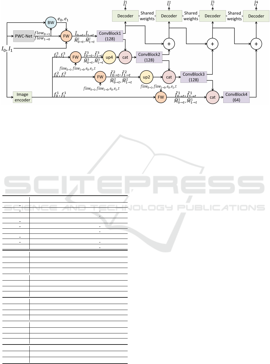
Figure 1: Overall architecture of our proposed method. Given two consecutive frames I

and I

, the ﬂow estimator ‘PWC-

Net’ and the feature extractor ‘Image encoder’ respectively predict bidirectional optical ﬂows flow

0→1

, flow

1→0

and extract

three-scale feature maps {f

, f

}. Backward Warping (BW) is ﬁrstly applied by taking source frames and

predicted ﬂows to output warping errors e

and e

which are used as conﬁdence measures. Then the Forward Warping (FW)

projects the input frames and their features to the desired time instant t, where the error maps e

and e

are used to handle

pixel overlaps. The feature maps in different scales bringing different levels of details are fed into ConvBlocks which generate

residues that are used to progressively reﬁne the feature volumes from the previous level (except for the lowest level). Finally,

a shared decoded reconstruct a set of intermediate frames with increasing levels of details. Please refer to Table 1 for the

detailed network architecture.

Table 1: Proposed network architecture. k, s and in/out

represent the kernel size, the stride and the number of in-

put/output channels, whereas ‘↑’ and ‘{}’ represent bilinear

upsampling and concatenation.

Encoder k s in/out input

conv1 1 3 1 3/128 I

or I

conv1 2 3 1 128/128 conv1 1

or f

3 1 128/128 conv1 2

conv2 1 3 2 128/128 f

or f

conv2 2 3 1 128/128 conv2 1

or f

3 1 128/128 conv2 2

conv3 1 3 2 128/128 f

or f

conv3 2 3 1 128/128 conv3 1

or f

3 1 128/128 conv3 2

ConvBlock1

convA1 3 1 8/128 {

0→t

1→t

0→t

1→t

}

convA2 3 1 128/128 convA1

3 1 128/128 convA2

ConvBlock2

convB1 3 1 322/128 {↑(

0→t

1→t

0→t

1→t

),R

}

convB2 3 1 128/128 convB1

3 1 128/128 convB2

ConvBlock3

convC1 3 1 322/128 {↑(

0→t

1→t

0→t

1→t

),R

}

convC2 3 1 128/128 convC1

3 1 128/128 convC2

ConvBlock4

convD1 3 1 322/64 {↑(

0→t

1→t

0→t

1→t

),R

}

convD2 3 1 64/64 convD1

3 1 64/64 convD2

Decoder

convE1 3 1 64/64

n=1

3 1 64/3 convE1

warping error:

argmin

−

0→t

+ |I

−

1→t

, (2)

where

0→t

and

1→t

are respectively warped images

from given instants 0 and 1 to instant t.

There are actually two ways to obtain warped im-

ages

0→t

and

1→t

based on flow

0→1

and f low

1→0

One is to apply an ‘Image spatial transformation’ (or

Backward Warping (BW)) as used in (Jaderberg et al.,

2015). However, this requires interpolating f low

t→0

and f low

t→1

, as in (Jiang et al., 2018), before warp-

ing the images. However, interpolating intermediate

optical ﬂows always brings errors, especially at the

object boundaries. One can instead apply Forward

Warping (FW) in a similar way as in (Niklaus and Liu,

2020) or (Shi et al., 2020), which can directly warp

images to the time instant t without prior estimation

of f low

t→0

and f low

t→1

. However, the method in

(Shi et al., 2020) requires a prior ﬂow (depth maps

in the case of the approach in (Shi et al., 2020)) es-

timation for handling overlaid pixels after warping.

Overlaid pixels from foreground are given more im-

portance than those from background when interpo-

lating the ﬁnal pixel color values.

In order to compute a measure of conﬁdence for

the warped pixels, without having to interpolate the

optical ﬂows computed between the input frames, we

can, as in (Niklaus and Liu, 2020) instead calculate

Deep Video Frame Rate Up-conversion Network using Feature-based Progressive Residue Reﬁnement

333

brightness errors e

and e

to tackle pixel overlaps, as

RGB

− BW (I

, f low

0→1

)|, (3)

RGB

− BW (I

, f low

1→0

)|. (4)

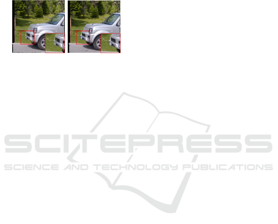
(a) Warped image be-

fore FT

(b) Warped image after

Figure 2: Visualization of

0→t

(a) before/ (b) after ﬁnetun-

ing (FT) ﬂow estimator.

Warping errors e

and e

are actually effective

cues for handling overlaps, since pixels coming from

occluded regions have larger error values than those

from visible regions, and these occluded pixels are

also more likely to be overlaid after warping. So, al-

though we use FW instead of BW to warp the input

frames to the intermediate time instant t, we use BW

for calculating e

and e

in Eq. 3 and Eq. 4.

With e

and e

, the authors in (Niklaus and Liu,

2020) further employ a U-Net which takes these error

maps and source frames as inputs to predict impor-

tance maps for the following FW operation. How-

ever, using such a network only for predicting the

pixel conﬁdence measures implies additional param-

eters, and makes the ﬁne-tuning together with PWC-

Net and U-Net more complicated with risks of net-

work collapse.

To avoid the above problems, we instead directly

use the normalized error maps e

and e

as impor-

tance maps in the FW step to handle pixel overlaps.

We adopt a scale factor α and exponential function to

compute the pixel conﬁdence measure as exp(−α ∗

). When increasing the value of α, overlaid pixels

having smaller error values will be given more impor-

tance, hence will contribute more to the interpolation.

A larger value of α is favorable to videos that contain

large occlusions due to motion. In our experiments,

we use a testset that includes different types of mo-

tion, and we experimentally found that α = 1 can

generate satisfactory results.

Besides the normalization of warping errors, we

also explicitly detect disocclusion regions: after

warping, the pixel positions that do not have any pixel

falling in its neighbourhood, are identiﬁed as disoc-

cluded positions. These positions are set to 0 in the

corresponding binary mask

M, and all the others are

set to 1. Based on the error maps normalization and

on the detection of disocclusions, our FW can be sum-

marized as follows:

0→t

= F W (I

, f low

0→t

, α ∗ e

), (5)

1→t

= F W (I

, f low

1→t

, α ∗ e

), (6)

where flow

0→t

= t ∗ f low

0→1

and flow

1→t

= (1 −

t) ∗ flow

1→0

The disocclusion masks

0→t

and

1→t

are cru-

cial to our method, since they allow us to exclude un-

reliable pixels, which are not inpainted during warp-

ing, from the objective function Eq. 2. The new func-

tion used for ﬁnetuning the ﬂow estimator, after tak-

ing the binary masks into account, becomes

argmin

|(I

−

0→t

)∗

0→t

+|(I

−

1→t

)∗

1→t

(7)

The disoccluded pixels are inpainted in the Con-

vBlocks, and the masks are indicating the disocclu-

sion positions. Based on Eq. 7, PWC-Net can be op-

timized speciﬁcally for the view synthesis task. The

effectiveness of our ﬁnetuning procedure is illustrated

in Fig. 2, where before ﬁnetuning, we can observe se-

vere deformations of the license plate, and blurriness

due to optical ﬂow inaccuracy. After ﬁnetuning, the

deformation and blurriness issue is considerably alle-

viated. This is further analyzed in the ablation study

section.

Apart from the improvement of the ﬁnal recon-

struction quality, the ﬁnetuning of PWC-Net before

end-to-end training can effectively shorten global

training time and prevent network collapse. An-

other reason for recommending this ﬁnetuning pro-

cess is that when the network is not end-to-end train-

able, such as in (Niklaus and Liu, 2018), having a

synthesis-task optimized ﬂow estimator deﬁnitely im-

proves the ﬁnal performance.

2.3 Progressive Residual Reﬁnement

The next step is to retrieve the intermediate

frame

based on these bi-directional ﬂows

flow

0→1

, f low

1→0

optimized for interpolation.

According to Eqs. 5 and 6, the original frames

, I

and extracted features f

, f

are ﬁrst warped to

instant t to obtain

0→t

1→t

0→t

1→t

and their

corresponding binary masks

0→t

1→t

. Con-

vBlock1 ﬁrst takes warped images and their masks

and outputs a feature volume containing a base repre-

sentation of scene information, which we then reﬁne

by adding residue feature volumes based on warped

features

0→t

1→t

at different levels obtained with

kernels having different receptive ﬁelds. These fea-

tures aim at capturing subtle textures in the scene, to

VISAPP 2022 - 17th International Conference on Computer Vision Theory and Applications

334

26.42dB/0.9014 26.64dB/0.9070

27.83dB/0.9317 28.42dB/0.9422

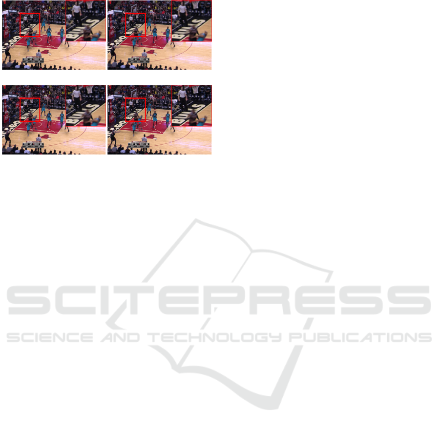
Figure 3: Visualization of progressively reﬁned details from

(from top to bottom, from left to right).

then reﬁne details of the base feature volume. The

merging of images resulting from both pixel-based

and feature-based warping has been shown power-

ful in (Shi et al., 2020) in the context of light ﬁeld

view synthesis. The features extracted at three dif-

ferent scales are used, via ConvBlock2-4, to learn

residues to progressively reﬁne the base feature map

volume. ConvBlock1-4 are three-layer convolutional

blocks. The last layer of ConvBlock1-3 is split into

two branches, one branch keeping a subset of fea-

tures that reﬁnes the previous level, while the sec-

ond subset of features (corresponding to higher fre-

quency details) is used at the next reﬁnement level

(see Fig 1(c)). Finally, a shared decoder is employed

to decode both the base volume and volumes progres-

sively reﬁned at different levels to obtain synthesized

views

(i = 1, 2, 3, 4). Fig. 3 shows this progres-

sive reﬁnement from

. From

, more

and more details are added and artefacts are gradually

corrected. We use

as our ﬁnal interpolated frame

as it contains the most details. The whole pipeline

is trained by minimizing the following reconstruction

error:

rec

i=1

Lap(I

−

), (8)

where Lap is the Laplacian loss (Bojanowski et al.,

2017) with three levels, and λ

are hyperparameters

for controlling the reconstruction quality at each level.

More precisely, we set λ

to non-zero values at the

beginning of the training, to enforce a target frame

reconstruction at each network level. Once each net-

work level is well initialized, we set λ

to non-zero

and the other λ values to zero in order to only focus

on the last reconstruction step.

3 TRAINING DETAILS

We use tensorﬂow to implement our method and

Adam to optimize the model with β

= 0.9 and

= 0.999. The overall training schedule of our

method is divided in two steps: ﬁrst ﬁnetuning PWC-

Net and then training the whole network.

The ﬁnetuning of PWC-Net aims at optimizing its

weights for the synthesis task. In this step, we set

the batch size to 20, the patch size to 160×160 and

the learning rate to 10

−4

to ﬁnetune PWC-Net for 20

epochs. We found that 20 epochs of ﬁnetuning can

already correct most of deformations and blurriness.

More epochs will prolong the overall schedule while

bringing limited improvement. We found that this

ﬁnetuning procedure is helpful to the global schedule,

since the following training procedure will be much

longer, and may suffer from performance oscillation

or even collapse without a ﬁnetuned ﬂow estimator.

The training of the whole network is made in two

steps. We ﬁrst ﬁx the weights in PWC-Net and update

the other variables, with a batch size of 20, a patch

size of 160×160, a learning rate of 10

−4

and λ

...λ

{0.1, 0.2, 0.4, 0.8} for 50 epochs. This step guides

the ConvBlock1-4 layers to learn residues for correct-

ing details in a coarse to ﬁne manner. In the sec-

ond step, we end-to-end train the network and update

all variables, with a batch size of 16, a patch size of

160×160, a learning rate of 10

−5

and λ

= 1 for 40

epochs. λ

, λ

are set to 0 to make the optimiza-

tion focus on the ﬁnal synthesized view. The training

of our pipeline has been conducted on a Nvidia Tesla

V100 GPU card with 32GB GRAM, and took about 6

days to converge.

4 EXPERIMENTAL RESULTS

We have carried out experiments on several datasets

and measured the PSNR and SSIM of the interpolated

frames in comparison with state-of-the-art methods.

4.1 Datasets

We used the following datasets:

• Training Dataset. Both ﬁnetuning of PWC-Net

and training of the network have been conducted

using the Vimeo90K training set (Xue et al.,

2019), which contains 51,312 frame triplets with

resolution 256×448. We use the ﬁrst and the last

frames as inputs and the intermediate frame as

ground truth.

• Test Datasets. We have used two test sets to as-

sess the quality of the synthesized frames: 1) the

Deep Video Frame Rate Up-conversion Network using Feature-based Progressive Residue Reﬁnement

335

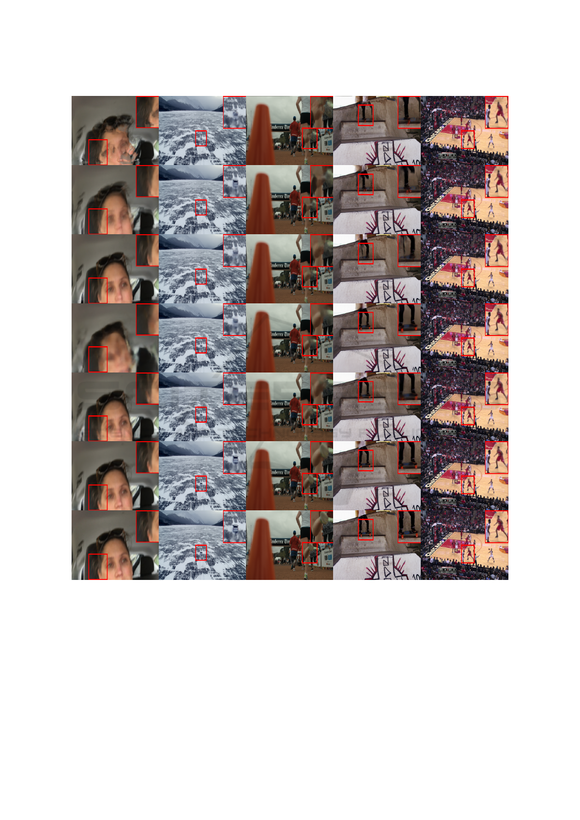
Figure 4: Visual comparison of synthesized frames for different methods. From top to bottom, they are frames interpolated

using SuperSloMo (Jiang et al., 2018), SepConv (Niklaus et al., 2017b), MEMC (Bao et al., 2019b), FeFlow (Gui et al., 2020),

SMSP (Niklaus and Liu, 2020), Our method. The last row shows ground truth frames.

Vimeo90K testset which has 3,782 frame triplets

with resolution 256×448; 2) the Adobe240fps

dataset is a dataset captured by a handheld cam-

era. We have extracted 777 frame triplets and in-

terpolated the intermediate frame during testing.

4.2 Experimental Set Up

We compare the proposed video frame interpola-

tion method with the most representative and recent

methods: SuperSloMo (Jiang et al., 2018), SepConv

(Niklaus et al., 2017b), MEMC (Bao et al., 2019b),

FeFlow (Gui et al., 2020) and SMSP (Niklaus and

VISAPP 2022 - 17th International Conference on Computer Vision Theory and Applications

336

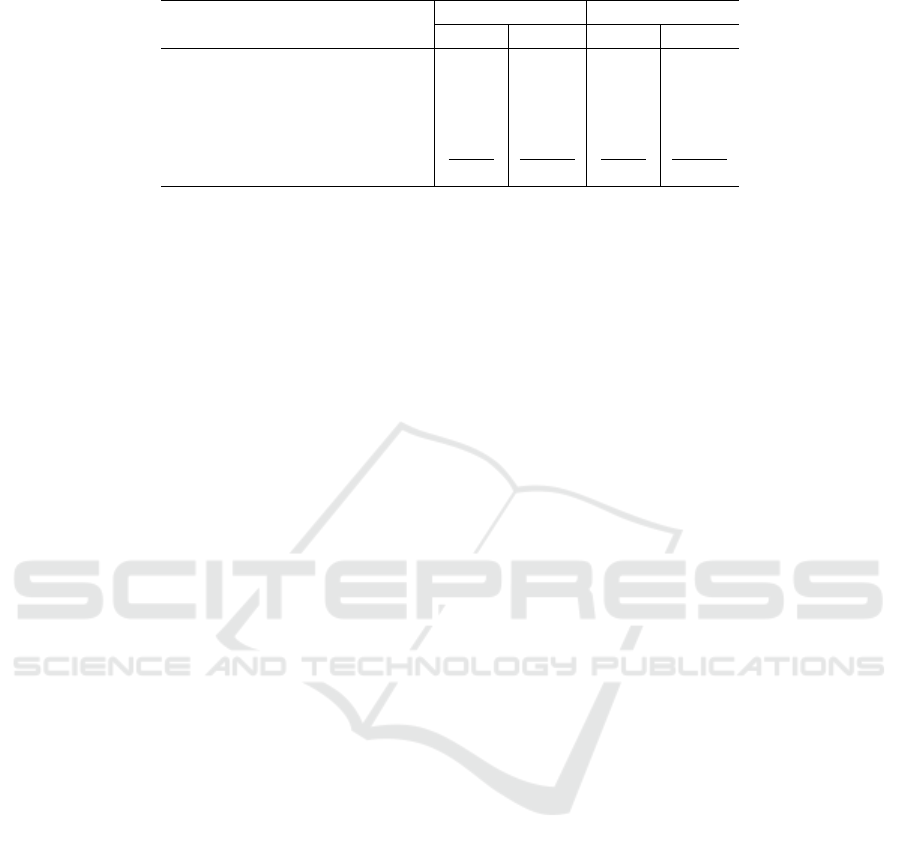
Table 2: Quantitative results (PSNR&SSIM) for the interpolated frames (averaged over 3782 and 777 frames).

Methods

Vimeo90K Adobe240fps

PSNR SSIM PSNR SSIM

SuperSloMo(Jiang et al., 2018) 30.92 0.9320 28.44 0.8966

SepConv(Niklaus et al., 2017b) 33.80 0.9555 31.16 0.9225

MEMC(Bao et al., 2019b) 34.43 0.9625 31.54 0.9269

FeFlow(Gui et al., 2020) 35.09 0.9629 31.50 0.9248

SMSP(Niklaus and Liu, 2020) 35.49 0.9671 31.62 0.9269

Ours 35.86 0.9689 31.80 0.9286

Liu, 2020). Among them, SuperSloMo infers the op-

tical ﬂow in the target instant to backward project the

input frames and employs soft visibility maps to han-

dle occlusions. SepConv formulates the frame inter-

polation problem as a local separable convolution us-

ing 1D kernels. Target frames are synthesized with-

out involving any optical ﬂow. MEMC predicts both

optical ﬂows and convolution kernels respectively for

global motion estimation and local motion compen-

sation in its synthesis process. FeFlow pioneers the

ﬂows of feature maps instead of images to retrieve an

intermediate frame. SMSP builds a two-stage syn-

thesis pipeline by using an off-the-shelf PWC-Net for

ﬂow prediction, and a GridNet (Fourure et al., 2017)

for frame synthesis, which is in the same vein as ours.

For a fair comparison, we use the ofﬁcial authors’

implementations for the methods SepConv (Niklaus

et al., 2017b), MEMC (Bao et al., 2019b) and FeFlow

(Gui et al., 2020). We use a third-party code and a

pre-trained model for the SuperSloMo (Jiang et al.,

2018) method. For the SMSP method (Niklaus and

Liu, 2020), the authors only provide the implementa-

tion of their FW operation. The rest of the network

implementation and the trained models are not avail-

able. Therefore, we re-implemented and trained their

network architecture by following the instructions in

the paper. Since MEMC, FeFlow and SMSP are al-

ready trained on Vimeo90K dataset and SuperSloMo

is trained on Adobe240fps datasets, we use the default

parameter settings recommended by the authors in our

experiments, e.g. we use kernel size 4 × 4 in adaptive

warping layer of MEMC, 16 groups of attention maps

in FeFlow etc.

4.3 Interpolation Results

The performances of all tested methods are shown in

Table 2. We can observe that our method outperforms

the best referenced methods by a margin of about 0.2-

0.3dB. This gain of PSNR is not trivial, as we can

notice that the difference in terms of PSNR between

the reference methods is sometimes less than 0.1dB.

Besides the quantitative evaluation in terms of

PSNR and SSIM, Fig 4 shows synthesized views us-

ing different methods. We zoomed regions contain-

ing subtle details in each image for comparison. We

can notice that our method better reconstructs details

when compared with other methods. For details like

the hair in the ﬁrst scene and the car in the second

scene, where other methods suffer from a deforma-

tion or blurriness, our pipeline yields more plausible

results.

Another advantage of our method is that it can

up-convert videos to an arbitrary frame rate, since

the target instant t can be any value between 0

and 1. Methods such as SepConv and FeFlow can

only interpolate frames at t = 0.5, which means

that, to interpolate by a factor of N = 2

(k >

1), they must recursively perform k interpolations.

Interpolation errors will gradually augment during

this recursive synthesis process. We have 8X up-

converted video frame rate using different methods,

and the corresponding interpolated videos can be

found in our project homepage: http://clim.inria.fr/

research/VISAPP2022/index.html, where high frame

rate videos obtained using our pipeline have less arti-

facts and deformations than others.

Please note that, like most of the frame synthesis

methods, our method is based on linear-motion as-

sumption, all motions are supposed to have uniform

velocities during frame warping process. Inferring

both velocity and acceleration of motion using only

two frames is a very ill-posed problem, it is more in-

vestigated in a multi-frame (Bao et al., 2018; Reda

et al., 2019; Xu et al., 2019) context.

4.4 Ablation Study

4.4.1 Forward Warping Method

Although both our method and SMSP are built on

PWC-Net, the rest of the network has a different de-

sign. In SMSP, the authors employ a neural network

that takes brightness errors e

, e

in Eq.3 and Eq.4 to

learn maps of importance for handling pixel overlaps,

this network increases the total parameter number but

brings little improvement. While we normalize two

brightness errors as maps of importance, which is

Deep Video Frame Rate Up-conversion Network using Feature-based Progressive Residue Reﬁnement

337

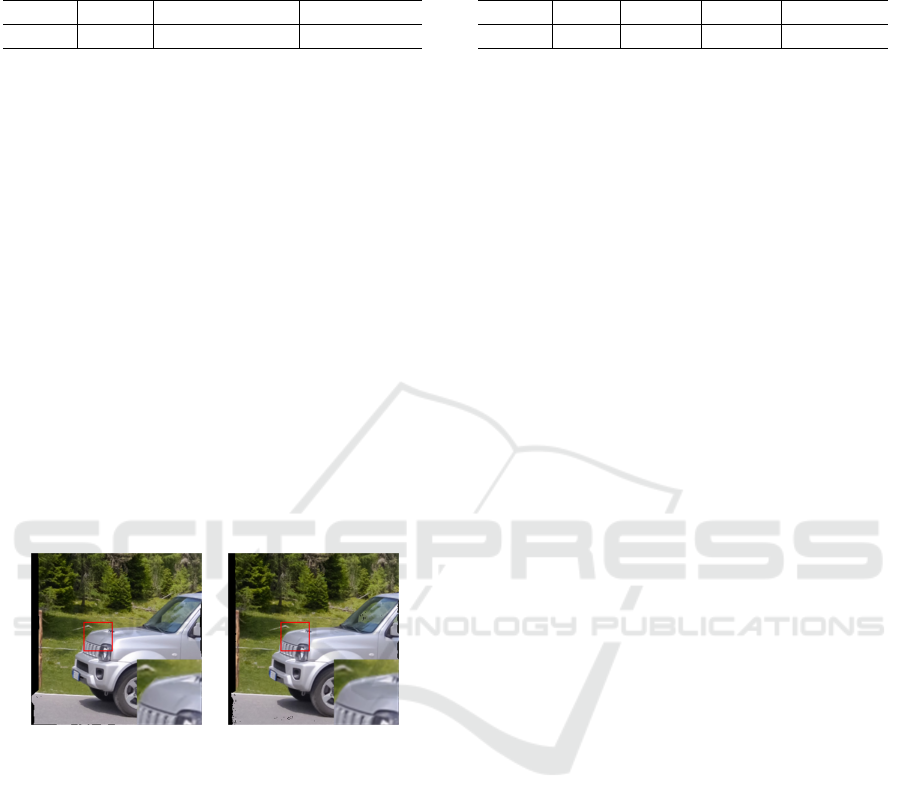
Table 3: Quantitative evaluation of different ﬁnetuning

strategies on Vimeo90K testset. The obtained PSNR val-

ues are averaged over 3782 frames.

Types wo FT FT(SMSP FW) FT(our FW)

PSNR 31.26 33.38 33.81

likewise effective in handling pixel overlaps but with-

out an increasing parameter number.

Fig. 5 shows the warped images obtained when us-

ing the FW step proposed in SMSP (Niklaus and Liu,

2020). Although the quality of the two warping meth-

ods looks similar, the proposed method is very simple,

as it does not use extra network as in (Niklaus and

Liu, 2020). We have also quantitatively evaluated the

performance when using different FW strategies. Ta-

ble 3 shows averaged PSNR over 3782 frames. More

specially, we use optical ﬂows to warp the ﬁrst and

the third frames to the intermediate instant, and com-

pare it with ground truth frame. In this process, all

disoccluded pixels are excluded. The employed op-

tical ﬂows are estimated without ﬁnetuning or with

ﬁnetuning, using FW proposed in (Niklaus and Liu,

2020), or ﬁnetuned using our proposed FW. Our pro-

posed simple FW step makes the end-to-end ﬁne tun-

ing of all the network components of the architecture

easier, leading to a better quality for the ﬁnal interpo-

lated frames.

(a) Warped image us-

ing FW proposed in

(Niklaus and Liu, 2020)

(b) Warped image using

our proposed FW

Figure 5: Visualization of

0→t

using (a) FW proposed in

(Niklaus and Liu, 2020) and (b) Our FW.

4.4.2 Reﬁnement Structure and Parameters

Compared with the complex GridNet model of (Fou-

rure et al., 2017), our progressive reﬁnement block

is simple but efﬁcient, it focuses more on the details

of the retrieved frames. Fine details are better re-

constructed with the help of learned residues. Using

fewer parameters (1.9M vs 3.0M), our method ﬁnally

achieves better performance (in Table 2) and visual

quality (in Fig.4) than SMSP.

To investigate the impact of using multi-levels re-

ﬁnement, we carry out experiments either using only

the base layer (with the warped input frames only),

Table 4: Quantitative evaluation of different levels of reﬁne-

ment. The obtained PSNR values are averaged over 3782

frames of the Vimeo90K testset.

Types base 1-layer 2-layer full model

PSNR 35.05 35.19 35.40 35.86

or using one, two, or three levels of reﬁnement of

the warped images features. Table 4 shows averaged

PSNR values when adopting different levels of reﬁne-

ment. The full model using three layers of reﬁnement

gives the best performance.

5 CONCLUSION

In this work, we proposed a ﬂow-based network ar-

chitecture that uses deep features to progressively re-

ﬁne a temporally interpolated frame in a context of

video frame rate up-conversion. We also proposed

a novel ﬁnetuning procedure that optimizes ﬂow es-

timation networks for the interpolation task without

using any ground truth optical ﬂows. A comprehen-

sive qualitative and quantitative assessment on differ-

ent video frame interpolation datasets shows that our

method can generate high quality interpolated frames

with realistic details.

REFERENCES

Bao, W., Lai, W., Ma, C., Yang, M., et al. (2019a). Depth-

aware video frame interpolation. In IEEE. Int. Conf.

on Computer Vision and Pattern Recognition (CVPR),

pages 3703–3712.

Bao, W., Lai, W., Zhang, X., Yang, M., et al. (2019b).

Memc-net: Motion estimation and motion compensa-

tion driven neural network for video interpolation and

enhancement. IEEE Trans. Pattern Anal. Mach. Intell.

(TPAMI).

Bao, W., Zhang, X., Chen, L., Ding, L., and Gao, Z.

(2018). High-order model and dynamic ﬁltering for

frame rate up-conversion. IEEE Trans. Image Proc.

(TIP), 27(8):3813–3826.

Bojanowski, P., Joulin, A., Lopez-Paz, D., and Szlam, A.

(2017). Optimizing the latent space of generative net-

works. arXiv preprint arXiv:1707.05776.

Butler, D. J., Wulff, J., Stanley, G. B., and Black, M. J.

(2012). A naturalistic open source movie for opti-

cal ﬂow evaluation. In Eu. Conf. on Computer Vision

(ECCV), pages 611–625.

Choi, M., Kim, H., Han, B., Xu, N., and Lee, K. (2020).

Channel attention is all you need for video frame in-

terpolation. In AAAI Conference on Artiﬁcial Intelli-

gence, pages 10663–10671.

Dosovitskiy, A., Fischer, P., Ilg, E., et al. (2015). Flownet:

Learning optical ﬂow with convolutional networks. In

IEEE Int. Conf. on Computer Vision (ICCV).

VISAPP 2022 - 17th International Conference on Computer Vision Theory and Applications

338

Fourure, D., Emonet, R., Fromont, E., et al. (2017). Resid-

ual conv-deconv grid network for semantic segmenta-

tion. In British Machine Vision Conf. (BMVC).

Gui, S., Wang, C., Chen, Q., and Tao, D. (2020). Fea-

tureﬂow: Robust video interpolation via structure-

to-texture generation. In IEEE. Int. Conf. on Com-

puter Vision and Pattern Recognition (CVPR), pages

14004–14013.

Hui, T., Tang, X., and Loy, C. C. (2018). Liteﬂownet: A

lightweight convolutional neural network for optical

ﬂow estimation. In IEEE. Int. Conf. on Computer Vi-

sion and Pattern Recognition (CVPR), pages 8981–

8989.

Ilg, E., Mayer, N., Brox, T., et al. (2017). Flownet 2.0: Evo-

lution of optical ﬂow estimation with deep networks.

In IEEE. Int. Conf. on Computer Vision and Pattern

Recognition (CVPR), pages 2462–2470.

Ilg, E., Saikia, T., Keuper, M., and Brox, T. (2018). Oc-

clusions, motion and depth boundaries with a generic

network for disparity, optical ﬂow or scene ﬂow esti-

mation. In Eu. Conf. on Computer Vision (ECCV).

Jaderberg, M., Simonyan, K., Zisserman, A., et al. (2015).

Spatial transformer networks. In Advances in Neural

Information Processing Systems (NIPS), pages 2017–

2025.

Jiang, H., Sun, D., Jampani, V., Kautz, J., et al. (2018).

Super slomo: High quality estimation of multiple in-

termediate frames for video interpolation. In IEEE.

Int. Conf. on Computer Vision and Pattern Recogni-

tion (CVPR), pages 9000–9008.

Liu, Z., A, R. Y., Tang, X., Liu, Y., and Agarwala, A.

(2017). Video frame synthesis using deep voxel ﬂow.

In IEEE Int. Conf. on Computer Vision (ICCV), pages

4463–4471.

Meyer, S., Djelouah, A., McWilliams, B., Schroers, C.,

et al. (2018). Phasenet for video frame interpolation.

In IEEE. Int. Conf. on Computer Vision and Pattern

Recognition (CVPR), pages 498–507.

Meyer, S., Wang, O., Zimmer, H., Sorkine-Hornung, A.,

et al. (2015). Phase-based frame interpolation for

video. In IEEE. Int. Conf. on Computer Vision and

Pattern Recognition (CVPR), pages 1410–1418.

Niklaus, S. and Liu, F. (2018). Context-aware synthesis for

video frame interpolation. In IEEE. Int. Conf. on Com-

puter Vision and Pattern Recognition (CVPR), pages

1701–1710.

Niklaus, S. and Liu, F. (2020). Softmax splatting for video

frame interpolation. In IEEE. Int. Conf. on Computer

Vision and Pattern Recognition (CVPR), pages 5437–

5446.

Niklaus, S., Mai, L., and Liu, F. (2017a). Video frame inter-

polation via adaptive convolution. In IEEE. Int. Conf.

on Computer Vision and Pattern Recognition (CVPR),

pages 670–679.

Niklaus, S., Mai, L., and Liu, F. (2017b). Video frame

interpolation via adaptive separable convolution. In

IEEE Int. Conf. on Computer Vision (ICCV), pages

261–270.

Reda, F., Sun, D., Dundar, A., Shoeybi, M., Liu, G., Shih,

K., Tao, A., Kautz, J., and Catanzaro, B. (2019).

Unsupervised video interpolation using cycle consis-

tency. In IEEE. Int. Conf. on Computer Vision and

Pattern Recognition (CVPR), pages 892–900.

Shi, J., Jiang, X., and Guillemot, C. (2020). Learning fused

pixel and feature-based view reconstructions for light

ﬁelds. In IEEE. Int. Conf. on Computer Vision and

Pattern Recognition (CVPR), pages 2555–2564.

Soomro, K., Zamir, A. R., and Shah, M. (2012). Ucf101:

A dataset of 101 human actions classes from videos in

the wild. arXiv preprint arXiv:1212.0402.

Sun, D., Yang, X., Liu, M., and Kautz, J. (2018). Pwc-

net: Cnns for optical ﬂow using pyramid, warping,

and cost volume. In IEEE. Int. Conf. on Computer

Vision and Pattern Recognition (CVPR), pages 8934–

8943.

Xu, X., Siyao, L., Sun, W., Yin, Q., and Yang, M. (2019).

Quadratic video interpolation. Advances in Neural In-

formation Processing Systems (NIPS).

Xue, J., Chen, B., T, W., et al. (2019). Video enhance-

ment with task-oriented ﬂow. Int. J. Computer Vision

(IJCV), 127(8):1106–1125.

Deep Video Frame Rate Up-conversion Network using Feature-based Progressive Residue Reﬁnement

339