Identiﬁcation of Planarian Individuals by Spot Patterns in Texture

Nikita Lomov

1 a

, Kharlampiy Tiras

2,3 b

and Leonid Mestetskiy

1,4 c

Federal Research Center “Computer Science and Control” of the Russian Academy of Sciences, Moscow, Russia

Institute of Theoretical and Experimental Biophysics of the Russian Academy of Sciences, Pushchino, Russia

Pushchino State Institute of Natural Science, Pushchino, Russia

Lomonosov Moscow State University, Moscow, Russia

Keywords:

Animal Identiﬁcation, Planarian Flatworms, Skeleton, Fat Curve, Point Registration, Assignment Problem.

Abstract:

Planarian ﬂatworms are known for their abilities to regenerate and are a popular biological model. Identi-

ﬁcation of individual planarian individuals is useful for automating biological research and improving the

accuracy of measurements in experiments. The article proposes a method for identifying planaria by their

texture proﬁle, characterized by a set, shape, and position of light spots on the worm’s body— areas without

pigment. To make the comparison of planaria of different sizes and in different poses, the method of planarian

texture normalization is suggested. It is based on the selection of a main branch in the skeleton of a segmented

image and allows one to switch to a uniﬁed coordinate system. Also, a method for creating a generalized

textural proﬁle of a planarian, based on averaging sets of spots for multiple images, is proposed. Experiments

were carried out to identify planaria for different types of observations—during one day, during several days

and during several days of regeneration after decapitation. Experiments show that light spots are a temporally

stable phenotypic trait.

1 INTRODUCTION

Freshwater ﬂatworms planaria are one of those groups

of animals that are recognized as classical biologi-

cal models. The ability of adult planarians to mor-

phogenesis, that is, regeneration and asexual repro-

duction (Bagu

a, 2012; Elliott and Alvarado, 2013;

Karami et al., 2015), is the most pronounced in the

animal kingdom. The only ones in the animal world,

planaria are even capable of regenerating their central

nervous system, the head ganglion, and this happens

in a very short time, from one to three weeks. The de-

velopment of digital technologies for the creation and

analysis of images has made it possible to develop a

quantitative description of the morphogenesis of pla-

naria in vivo (Tiras et al., 2015; Tiras et al., 2021).

Planarians are also one of the potentially promising

objects in the study of the cellular basis of immunity,

which in planarians proceeds by phagocytosis of food

by all planarian cells, except for nerve and germ cells

(Sheimann and Sakharova, 1974). Taking into ac-

count the current interest in various biological models

https://orcid.org/0000-0003-4286-1768

https://orcid.org/0000-0002-1853-8285

https://orcid.org/0000-0001-6387-167X

related to the problems of cellular immunity, planari-

ans can become one of the promising models for the

study of phagocytosis in vivo (Tiras et al., 2018; Peiris

et al., 2014; Apyari et al., 2021).

However, the widespread use of planaria for solv-

ing various fundamental and applied problems is hin-

dered by a number of unresolved objective problems,

one of which is the problem of identifying planarian

individuals in the course of an experiment. Thus, a

feature of the biology of the asexual race of planaria

Girardia tigrina is their preference for group habita-

tion during experiments. In addition, when seated

alone, planaria of this species tend to separate after 24

hours, which interferes with sufﬁciently long experi-

ments, therefore, during the experiment, such planari-

ans are kept in a group of 25-30 individuals in order to

limit asexual reproduction (Sheimann and Sakharova,

1974; Tiras et al., 2018). However, with group keep-

ing, it is impossible to distinguish planaria from each

other, which limits the possibility of assessing the in-

dividual characteristics of the course of certain physi-

ological processes over a number of days.

In this work, an attempt was made to identify pla-

naria based on the features of their body surface tex-

ture. The species name of the planaria, Girardia tig-

Lomov, N., Tiras, K. and Mestetskiy, L.

Identiﬁcation of Planarian Individuals by Spot Patterns in Texture.

DOI: 10.5220/0010802000003124

In Proceedings of the 17th International Joint Conference on Computer Vision, Imaging and Computer Graphics Theory and Applications (VISIGRAPP 2022) - Volume 4: VISAPP, pages

87-96

ISBN: 978-989-758-555-5; ISSN: 2184-4321

rina, is due to the patchy structure of their surface,

which is associated with the mosaic distribution of the

pigment epithelium. This circumstance opens up the

possibility of using the features of the body surface

texture of individual planarians as the basis for their

personal identiﬁcation.

Such an opportunity will make it possible to as-

sess the dynamics of morphogenesis and phagocyto-

sis of planaria in vivo, which will open up the pos-

sibility of creating quantitative models of the course

of these biological processes. Such models, in turn,

will be useful in studying the possibilities of control-

ling complex biological processes at the level of the

whole organism.

2 RELATED WORK

The identiﬁcation of individuals is an important task

for researchers in population ecology, ethology, bio-

geography and experimental biology. Although the

fundamental possibility of perfectly accurate identiﬁ-

cation is provided by DNA analysis, as well as the use

of chipping in combination with GPS tracking, it is

more realistic to use cheaper and non-invasive meth-

ods, for example, based on photography and video

surveillance. The rapid development of computer

vision systems observed in the last decade and the

strengthening of interdisciplinary interaction between

ﬁelds of science expressed in diffusion of methods

and approaches give hope for signiﬁcant progress in

this area. For example, popular methods of human

face recognition, pose estimation, and keypoint de-

tection, based on neural network models have been

successfully adapted to process individuals of higher

mammals of some species—brown bears (Clapham

et al., 2020), Amur tigers (Liu et al., 2019), chim-

panzees (Freytag et al., 2016).

A number of computer vision techniques using

hand-designed features have also been developed.

Depending on the particular species, the source of

signs can be stripes on the body for zebras (Lahiri

et al., 2011), dermal plates for turtles (Rao et al.,

2021), shape of the ﬁn for sharks (Hughes and

Burghardt, 2017), etc. In these cases, the feature

description can be presented in the form of vari-

ous mathematical objects: graphs, trajectories, point

clouds.

Particular individuals of animals, simpler than

mammals, are usually recognized insufﬁciently dis-

tinguishable, and the problem of recognizing various

closely related species, for example, worms (Lu et al.,

2021), is more often considered. It is one of the types

of worms, planarian ﬂatworms, that are object of our

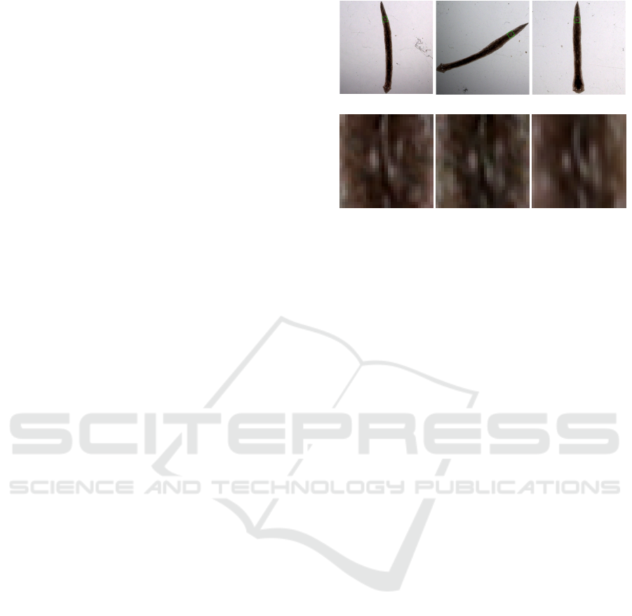
(a) (b) (c)

(d) (e) (f)

Figure 1: Planarian individual captured within a short pe-

riod of time (a-c) and a stable fragment of its texture (d-f).

The sources of this fragment are marked in (a-c) with green

frames.

interest. Planaria are versatile and powerful model

system for molecular studies of regeneration, adult

stem cell regulation, aging, and behavior. The fol-

lowing features of the planaria can be noticed from

the point of view of the task of visual recognition.

1. As their very name refers to, planaria are almost

ﬂat objects, and therefore their current appearance

is described with sufﬁcient completeness by a sin-

gle two-dimensional image.

2. Planaria have a signiﬁcant ability to bend, com-

press and stretch individual parts of the body, so

that their shape can be considered relatively rigid

only in the head region.

3. The coloration of planaria is very primitive and

does not allow the use of complex color charac-

teristics for the identiﬁcation of individuals.

4. Planaria are very dependent on environmental

conditions: the properties of the solution in which

they live, the weather outside the window, the diet

and the nature of the food they eat.

5. The body of a planarian is translucent, so the ap-

pearance in photographs is highly dependent on

shooting conditions and lighting.

The inﬂuence of these factors is illustrated in Fig.

1 showing the same planarian, photographed at dif-

ferent times. The distribution of body width in these

instances is very different: in Fig. 1a the thickness

of the planarian changes relatively slightly from the

tail to the head, in Fig. 1b the planarian has a strong

thickening about halfway, in Fig. 1c—severe thicken-

ing in the neck-like region above the head. At the

same time, on the body of the planarian, there are

fragments of a characteristic texture, which are pre-

served from photograph to photograph—Fig. 1d-e.

VISAPP 2022 - 17th International Conference on Computer Vision Theory and Applications

These are the same constellation of light spots—areas

marked by the absence of pigment. The idea of the al-

gorithm is to describe the texture of the planarian by

a set and location of the corresponding spots and to

organize the comparison procedure in such a way as

to include the search for mutual correspondence be-

tween spots in different photographs.

All these factors make the development of signif-

icant and stable feature of the appearance and shape

of planaria an urgent and challenging task. On the

other hand, like many other computer vision systems,

our approach will include several classical customary,

such as segmenting objects in an image, normalizing

their shape, and ﬁnding points of interest. They will

be discussed in the following sections.

3 OBJECT SEGMENTATION

(a) (b) (c)

(d) (e) (f)

Figure 2: Binarization stages.

Despite the fact that it is natural for planaria to live in

groups of 20-30 individuals, the quality of shooting

provided by the available microscope was not enough

to capture the entire group at once. Therefore, for

photographing, the planaria were moved one by one

into an intermediate vessel, and the segmentation task

was reduced to ﬁnding a single individual in the im-

age. Since most of the body of planaria is pigmented,

and they themselves live in a transparent solution, the

principle that planaria are darker than the background

(Fig. 2a) can be taken as the basis for binarization.

Nevertheless, it is necessary to take into account the

following conditions of shooting: ﬁrstly, due to the

distribution of light and optical effects, the brightness

of the image decreases towards its edges, and sec-

ondly, the walls of the vessel, which are also dark,

can get into the frame. Therefore, to normalize the

background, the morphological operation of opening

a grayscale image G with a disk of a ﬁxed diameter,

exceeding the width of the planarian, was performed

(Fig. 2b). Then the original image was subtracted

from the background and the negative of the result

was taken (Fig. 2c).

Next, the image was binarized using the Otsu

method, the average intensity values for the object

f g

∑

i j

<t]

∑

i j

<t]

and background µ

∑

i j

≥t]

∑

i j

≥t]

and binarization is performed with the threshold t

f g

+ 0.7(µ

−µ

f g

After that, the connected component with the

largest area is selected as the object mask. However,

since the walls of the vessel can be similar to a pla-

narian in size, color and shape, an additional check is

carried out: the sought component cannot touch the

edges of the image during Otsu binarization of the

original (without background subtraction) image. For

example, in Fig. 2d the red component will be as-

signed to the vessel walls, and the blue one will be

assigned to the background as a result of checking the

image in Fig. 2e. Also, to eliminate noise at the bor-

der with the ﬁnal component, an operation of mor-

phological opening is carried out, which gives us as a

result Fig. 2f.

4 MAIN AXIS EXTRACTION

Shape standardization is an important stage in solv-

ing problems related to the recognition of ﬂexible ob-

jects. It can be brieﬂy described as follows. Let there

be a segmented image B with an area D ⊂ R

to the object. It is required to ﬁnd the transforma-

tion T : D → Ω, where Ω ∈ R

is a standard domain.

Usually, additional requirements are imposed on the

transformation, for example, injectivity or smooth-

ness. Sometimes, if it is known that the form itself

is segmented into several parts {D

}, then the require-

ment p ∈ D

→ T (p) ∈ Ω

should be satisﬁed. For

instance, this setting is used in (Qu and Peng, 2010)

for standardizing confocal images of fruit ﬂy nervous

systems. As a rule, for standardization, a certain ref-

erence set is chosen, which is a curved axis of sym-

metry of an object or its part. So, this approach was

discussed in (Duyck et al., 2015) for straightening

species with strong bilateral symmetry such as mar-

bled salamanders, skinks and geckos. At the same

time, the situation with worms is relatively simple,

since their shape, in fact, appears to be the vicinity of

a single line.

Let this line be smooth and described by the

equation q(t) = (x(t),y(t)), t ∈ [0,l], and x

(t)

= 1. The tangent to this curve has the direction

u(t) = (x

(t),y

(t)), and the perpendicular is v(t) =

(t),−x

(t)). Let there also exist d, s.t. ∀p ∈ D ∃t ∈

[0,l] : ||p −q(t)|| ≤ d, and d <

max

t∈[0,l]

√

(t)

Identiﬁcation of Planarian Individuals by Spot Patterns in Texture

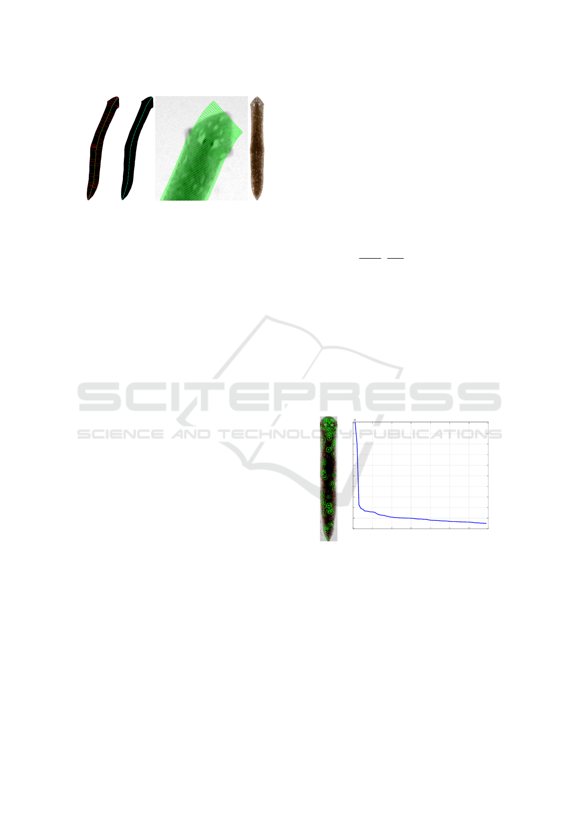
(a) (b) (c) (d)

Figure 3: Stages of main axis extraction.

Then the mapping

∗

(t,s) = (x(t)+(s−d)y

(t),y(t)−(s−d)x

(t)) (1)

is smooth, injective and maps the rectangle M =

[0,2d] ×[0, l] to the domain D

∗

⊃ D. Accordingly,

the transformation T = (T

∗

)

−1

maps D to the subset

of rectangle M, which, using scale transformations,

allows you to get a texture of a ﬁxed size.

To determine the desired main axis of the worm,

in the work (Peng et al., 2007) an approach, based

on dividing the border into nominally left and right

parts, highlighting the middle line as a sequence of

midpoints of segments when traversing the left and

right parts and then reﬁning the middle lines. Later

this algorithm was developed in (Flygare et al., 2013)

for better handling of worms of small eccentricity, i.e.

insufﬁciently elongated, with a shape close to elliptic.

To improve the algorithm, the coefﬁcient of asymme-

try was determined between the left and right regions

of the worm’s body, into which the medial axis di-

vides the shapes. Note that since we are essentially

dealing with the search for an extended curvilinear

axis of symmetry of the worm, it is natural to use the

model of continuous skeleton (or, synonymously, me-

dial axis) of binary image (Mestetskiy and Semenov,

2008). The skeleton consists of lines equidistant from

two or more sections of the boundary (all solid lines

in Fig. 3a) and contains the required axis as a sub-

graph. Obviously, the shape of the worm should be

restored with sufﬁcient completeness by the union of

the inscribed circles lying on the main axis—in fact,

we are talking about representing the worm’s shape

by a fat curve (Mestetskiy, 2000). Therefore, to se-

lect the base of the axis, the pruning of the skeleton

is performed—all branches of the skeleton that do not

make a signiﬁcant contribution to the formation of the

shape are removed (green line in Fig. 3a). On the

other hand, the main axis should stretch from the top

of the head to the tip of the tail. These points are de-

ﬁned as the points with the farthest projection on the

tangent rays to the ends of the base (dashed lines in

Fig. 3a), then the base is supplemented with paths in

the skeleton from the ends of the base to the found

points (blue lines in Fig. 3a).

To smooth the main axis, m points are sampled

evenly on it, which gives us a set of {x

}

m−1

k=0

where r

is the radius of the insribed circle centered

in (x

). Then, using piecewise cubic Hermitian in-

terpolation (Fritsch and Carlson, 1980), we obtain the

smoothed version of the main axis: {x(t),y(t),r(t)},

t ∈ [0,m −1] (Fig. 3b). Let also the maximum ra-

dius of the inscribed circle on the curve be r

max

. We

set d = r

max

, so that the normalized texture ﬁts into

the borders of the image. Then, for a texture of size

w ×h, a pixel with coordinates (i, j ) corresponds to

a point of the original image with the coordinates



(i, j) = T

∗

(

i(m−1)

h−1

j(2d)

w−1

), according to formula 1.

A fragment of the curvilinear grid is shown in Fig. 3c

and the straightened texture is shown in Fig. 3d. To

ﬁll the texture, bilinear interpolation was used, and

pixels in positions (i, j) for which T



(i, j) /∈ D were

unmasked by alpha channel.

5 SEARCH FOR POINTS OF

INTEREST

5.1 Spot Extraction

0 10 20 30 40 50 60 70

Rank

0.2

0.4

0.6

0.8

1.2

1.4

1.6

1.8

Strength

(a) (b)

Figure 4: SURF points with negative Laplacian value: lo-

cation (a) and strength sorted in descending order (b).

The surface of a planarian individual has a character-

istic pattern of light spots, that are the areas without

pigment. These spots are small in size and of prim-

itive, moreover, not always stable, shape. Although

one is able to match areas related to the same spots, in

different photographs of the same planaria, and also it

is intuitively clear what can be understood by “more

spotty” and “less spotty” planarians and parts of their

bodies, it is not possible to give an exact answer to the

question of how many spots are located on the body

VISAPP 2022 - 17th International Conference on Computer Vision Theory and Applications

Algorithm 1: Extraction of spots in texture.

Require: Grayscale image G, number of spots n, minimum

spot area s

min

, threshold step h

Ensure: Binary image B with spots

t = 1

B ← (G ∗LoG

) ≤

m ← #{CC(B,s

min

)}  m ← the number of conn.comp. of

B that are greater than s

min

if m = n then

Return

else if m < n then

while m < n do

t ←t + h

B ← (G ∗LoG

) ≤

m ← #{CC(B,s

min

)}

end while

else

while m > n do

t ←t −h

B ← (G ∗LoG

) ≤

m ← #{CC(B,s

min

)}

end while

B ← (G ∗LoG

) ≤

t+h

end if

Leave in B n largest connected components

of a particular planarian. The situation is illustrated

by Fig. 4, where SURF points of interest (Bay et al.,

2008), which are lighter than the neighborhood, de-

tected in the texture, are shown, along with the plot

of their saliency depending on the rank. The graph

shows that, with the exception of a few ﬁrst points, the

saliency changes very smoothly, which does not allow

setting an effective threshold rule due to a strong de-

crease in saliency. Moreover, the scalar products of

the feature vectors of these points are stably greater

than 0.5, and in more than half of the cases, exceed

0.9. This indicates that the main feature of spots is

their location, not their appearance, and also leads to

the idea of extracting a ﬁxed number of spots from an

arbitrary texture. For this purpose, we use the Lapla-

cian Gaussian ﬁlter:

LoG

(x,y) = −

πσ



1 −

+ y

2σ



exp



−

+ y

2σ



(2)

The spots will be deﬁned as connective components in

the binary image B = (G ∗LoG

) ≤t, with more than

half of the pixels belonging to the foreground. If the

image is too blurry, not enough contrast, or does not

contain a sufﬁcient number of obvious spots, we will

use the linearity and stability (

∑

LoG

(x,y) = 0)

of the ﬁlter:

(aG + b) ∗LoG

= a(G ∗LoG

and we will select the binarization threshold instead

of increasing the contrast of the image itself. An al-

gorithm based on this principle is presented as Algo-

rithm 1.

5.2 Localization of Eyes

Light spots can occur in arbitrary places on the body

of a planarian, from head to tail. However, there are

two areas, which are also marked by the absence of

pigment and stand out as spots, but which are invari-

ably present in speciﬁc places—these are the eyes of

the planarian. The selection of eyes is important for

several purposes, the main one of which is the orien-

tation of the planarian texture (determining the head

end by the presence of eyes in it is a more reliable

criterion than, say, a wider head end as compared to

the tail end). We will determine the eyes as the best,

in some sense, pair of spots extracted at the previous

stage. Let (a

) be the area, abscissa and ordinate

of the center of the i-th spot found in the texture of

size w ×h. We use the following geometric properties

of the eyes:

• the area of the eye is usually larger than the area

of the regular spot;

• the eyes are located close to the border of the tex-

ture vertically;

• are located approximately at the same vertical

level;

• are located symmetrically about the vertical line

dividing the texture in half.

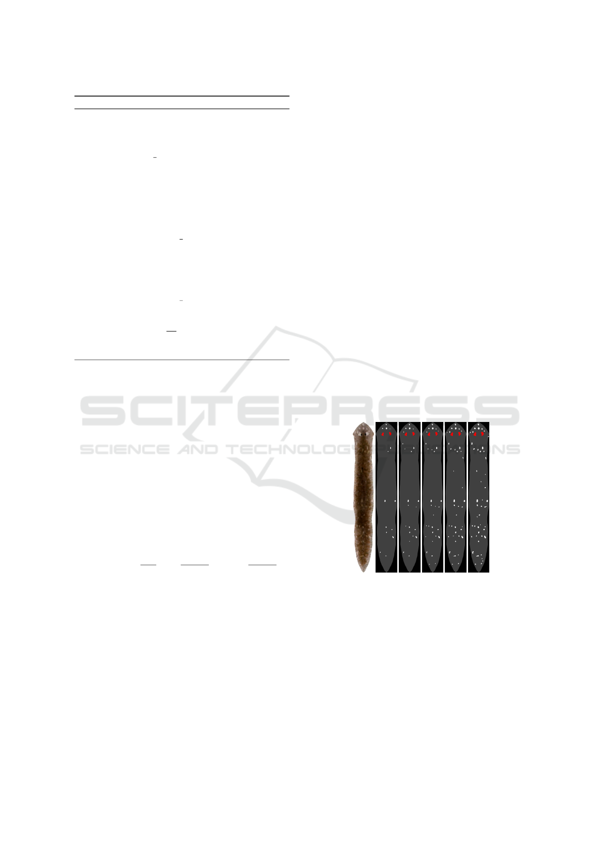
Texture n = 16 n = 24 n = 32 n = 40 n = 48

Figure 5: Extracting a different number of spots from a tex-

ture. Eye spots are highlighted in red.

For the spots with numbers (i, j), i 6= j we con-

struct the feature vector f

i j

containing the values

,min(y

,h −1 −y

),min(y

,h −1 −y

),y

−y

min(x

,w −1 −x

),min(x

,w −1 −x

),(x

+ x

−w + 1)}

and the monomes formed by them of order up to 3.

Then form a training sample from vectors of the form

−f

i j

with label 1 and f

i j

−f

with label −1, where

k and l refer to a pair of spots that are the eyes, and i

and j refer to the pair, marking no more than one eye.

Identiﬁcation of Planarian Individuals by Spot Patterns in Texture

SVM with a linear kernel is used for classiﬁcation and

when for the resulting model with weights w the pair

(t,s) maximizing hw,f

i is taken as the eyes. The

results of the extraction of the spots and the selection

of the eyes are shown in Fig. 5.

6 COMPARISON OF SPOT

PATTERNS

(a) (b) (c)

Figure 6: Assignment problem solutions for (a) pure match-

ing (task 3) (b) matching with L

-term with α = 15 used

(task 4) (c) matching of ordered sets (rule 5 involved).

Due to differences in lighting, bending, and living

conditions of planaria, it is rarely possible to isolate

completely coincident sets of spots. Therefore, when

looking for a match one need to take into account that

part of the spots is the noise. In (Qu and Peng, 2010)

this problem arises when comparing skin marks in the

evaluation of soft biometrics and is solved by leaving

in the list of matches only top-50% of the best pairs.

It is also possible to draw an analogy with the point

registration task, which is to ﬁnd the best match be-

tween two point clouds—ﬁxed X and moving Y. In

one of the most popular methods for solving it, co-

herent point drift (Myronenko and Song, 2010), the

problem is reduced to maximizing the likelihood

∏

i=1

p(x

), p(x) = w

+ (1 −w)

∑

m=1

p(x|m),

where p(x|m) =

(2πσ

)

D/2

exp

−||x−T (y

,θ)||

2σ

, and

T (Y,θ) is a transformation T applied to

Y = (y

,...,y

) and parameterized by θ. The

method provides a soft assignment of points to the

components of a mixture of Gaussians with centers

in X, and the weight w of the uniform distribution

actually sets the proportion of noise in the data. We

will look for a strict match between the spots of

textures, but some of the points will not be match at

all.

For two textures characterized by the sets p = {p

}

and q = {q

}, we deﬁne the matrix C ∈ R

n×n

: c

i j

d(p

), where d(p,q) is the dissimilarity measure

between spots. Let us deﬁne the dissimilarity between

sets as the minimum total dissimilarity between spots

in a one-to-one comparison, if only m ≤ n spots are

involved, which leads to the following task:

minimize

∑

i, j=1

i j

subject to

∑

i=1

i j

≤ 1 for i = 1,...,n,

∑

j=1

i j

≤ 1 for j = 1,...,n,

∑

i, j=1

i j

= m,

i j

∈ {0,1} for i = 1 ≤ i, j ≤ n.

(3)

This formulation is a variation of the classical as-

signment problem, which can be solved by one of the

integer linear programming methods, for example, the

branch and cut method.

Let us pay attention to the fact that the situa-

tion when the residual vectors (x(p

) −x(q

),y(p

) −

y(q

)) between the matched spots are similar to each

other is much more natural than the strong scatter in

these vectors. For example, when the tail of a pla-

narian is squeezed, all spots should move downward

in relative texture coordinates. Thus, a term can be

added to the functional that takes into account the

total deviation from the mean of the residual vec-

tors. In order not to go beyond the scope of the

linear programming problem, we will act in the L

metric. Let X ,Y ∈ R

n×n

, x

i j

= x(p

) − x(q

), and

i j

= y(p

) −y

(

). Then, for example, the deviation

from the average along the Y -axis takes the form:

∑

i=1

∑

j=1

i j



i j

−

∑

i, j=1

i j



Using the relaxing variables δ

,γ

∈R,i = 1,.. . , n,

the problem can be rewritten as:

minimize

∑

i, j=1

i j

+ α

∑

s=1

+ β

∑

t=1

subject to

∑

i=1

i j

≤ 1 for i = 1,...,n,

∑

j=1

i j

≤ 1 for j = 1,...,n,

∑

i, j=1

i j

= m,

VISAPP 2022 - 17th International Conference on Computer Vision Theory and Applications

∑

i=1

i j

−

∑

i, j=1

i j

−δ

≤ 0 for i = 1,...,n,

∑

i=1

i j

−

∑

i, j=1

i j

−γ

≤ 0 for i = 1,...,n,

i j

∈ {0,1} for i = 1 ≤ i, j ≤ n,

≥ 0,γ

≥ 0 for i = 1,...,n,

(4)

It can also be noted that, under possible defor-

mations of the planarian, the ordering of spots along

the Y -axis in the texture as a whole should be pre-

served. This property can be used in the formulation

of the functional, considering the ordered sets p and

q: i < j ⇒ y(p

) ≤ y(p

) & y(q

) ≤ y(q

) and adding

the following requirement to the 3 statement:

i j

= 1 & a

= 1 & i < s ⇒ j < t. (5)

The corresponding problem can be solved by dynamic

programming methods with recursive search for op-

timal matching k from l bottom spots. Visualiza-

tion of various methods of comparison for d(p,q) =

9(x(d) −x(q))

+ (y(d) −y(q))

is shown in Fig. 6.

7 GENERATION OF STANDARD

PATTERNS

Algorithm 2: Standard spot pattern calculation.

Require: Set of k sets of spots {p

= {p

i j

}

j=1

}

i=1

Ensure: Set of standard spots q = {q

}

i=1

Construct graph G = hV, Ei, where V is a set of all spots

in B and E is a set of all matches between spots in all

pairs in B

for i ← 1 to n do

← {v

}, v

= argmax

v∈V

#{e ∈ E : v ∈ e}

repeat

← {v ∈V \V

| ∃e = (v,v

) ∈ E : v

∈V

}

←V

∪V

until |V

| ≥ k or V

while |V

| > k do

← arg min

v∈V

#{e = (v,v

) ∈ E : v

∈V

}

←V

\{v

}

end while

for v ∈V

w(v) = #{e = (v, v

) ∈ E : v

∈V

}

f(v) is the feature vector of v

end for

←

∑

v∈V

w(v)f(v)

∑

v∈V

w(v)

V ←V \V

E ← E \{e ∈ E | e ∩V

end for

When solving the classiﬁcation problem by searching

for the most similar texture among the standards, it is

necessary to carry out a comparison procedure with

each of the class samples in the database, which can

turn out to be a time-consuming task. Naturally, the

need arises to create a generalized set of spots that

would best characterize the entire class and would be

similar to all available samples at once. Obviously,

this set should consist of spots that are stably detected

from image to image, and such spots in different im-

ages will most likely be matched to each other. If we

represent the structure of correspondence of points in

textures in the form of a graph, then due to the absence

of connections between points of the same image, the

task will become similar to analyzing a k-partite graph

in order to ﬁnd a clique (Dawande et al., 2001; Barber

et al., 2017) or a dense subgraph (Lee et al., 2010).

(a) (b) (c) (d) (e) (f) (g) (h) (i) (j)

Figure 7: Standard spot pattern generation. (a-h) Source

images, (i) locations of matched spots and (j) the resulting

standard. Some groups of matched spots are shown in spe-

ciﬁc colors.

To achieve a high speed of the procedure, a heuris-

tic algorithm of searching for a dense subgraph is pro-

posed based on expanding the neighborhood of a ver-

tex with a large number of connections and calculat-

ing the feature vector of a standard spot by averaging

the features of the vertices in the neighborhood. The

course of the procedure is described as Algorithm 2,

and its results are shown in Fig. 7.

8 EXPERIMENTS

8.1 Parameter Selection

The experiments were carried out with the following

parameters:

• number of points for main axis interpolation m =

64;

• texture height h = 1024;

• texture width w = 144;

• Gaussian ﬁlter deviation σ = 5;

Identiﬁcation of Planarian Individuals by Spot Patterns in Texture

• minimum spot area s

min

= 10;

• spot dissimilarity d(p,q) = 9(x(d) − x(q))

(y(d) −y(q))

For the experiments, the original datasets collected in

the laboratory of Pushchino State Institute of Natural

Science were used. Datasets are collections of im-

ages of size 1388 ×1080 obtained from photographs

taken with a Zeiss Stemi2000 binocular microscope

equipped with an AxioCam MRc video camera. The

ﬁrst set (“Day”) consists of images of entire planari-

ans, each of which was captured multiple times over

a limited period of time, not exceeding an hour. The

dataset contains a total of 1,764 images, with 28 sam-

ple classes, ranging from 16 to 113 images. The dis-

tribution of the length, understood as the length of the

main axis, and the area of the instances of the ﬁrst

15 classes from the dataset are shown in Fig. 8. The

graphs show that the ability of a planarian to shrink,

stretch and bend leads to a standard deviation of up

to 10% of the mean in length, and up to 8% in area.

For this reason, even the dimensions of a planarian

are difﬁcult to consider as a stable and discriminative

feature of the individual.

4 5 6 7 8 9 10

Length, mm

Area, mm

4.5 5 5.5 6 6.5 7 7.5 8 8.5 9 9.5

Length, mm

Area, mm

(a) (b)

Figure 8: Distribution of sizes in the “Day” dataset: (a)

individual instances and (b) standard deviations along to the

axis of PCA.

In order to investigate the inﬂuence of the num-

ber of spots—total and matched—on the identiﬁca-

tion accuracy, a part of this dataset was taken, con-

sisting of 16 images per class. The four earliest im-

ages from the class formed a training set, the 12 most

recent were used for testing. The nearest neighbor

algorithm was utilized for identiﬁcation, and the cor-

respondence of the points was established according

to formula 3, since the procedure it deﬁnes provides

the highest speed. The experimental results for a dif-

ferent number of selected spots n and matched spots

k are shown in Table 1 and allow us to conclude that

the quality of the method depends rather on the pro-

portion of the compared spots than on their absolute

number. In what follows, we set n = 24 and k = 12 as

the parameters that showed the best quality.

Table 1: Classiﬁcation accuracy for the ”Day” dataset with

a different number of selected and matched spots.

Total

Matched

6 8 10 12 16 20 24 28

16 90.48% 95.83% 95.83% 91.96% 33.33% − − −

20 91.96% 96.43% 98.51% 98.81% 91.07% 39.29% − −

24 91.07% 95.83% 97.32% 98.81% 97.32% 88.69% 42.86% −

28 89.29% 96.13% 97.62% 98.81% 98.51% 97.32% 84.82% 45.24%

32 86.01% 91.96% 95.24% 96.73% 98.21% 98.51% 96.73% 83.93%

36 84.82% 90.18% 94.05% 96.43% 98.21% 98.21% 97.62% 95.54%

40 80.95% 87.50% 91.67% 94.35% 96.73% 98.51% 97.92% 97.32%

8.2 Comparison of Matching Methods

The full “Day” dataset was considered, 10% of the

images of each class were used as training, the rest

were used as test. The following spot matching meth-

ods discussed in the Section 6 were compared:

• assignment problem solution without additional

terms (formula 3)—AP (plain);

• assignment problem solution with L

-norm on the

deviation from the mean (formula 4, α = 15, β =

5)—AP (L

-norm);

• assignment problem solution with y-ordering pre-

served (formula 5)—AP (y-ordered);

• coherent point drift (Myronenko and Song,

2010)—CPD.

Also, the same number of SURF points was high-

lighted as points of interest. To be consistent with all

matching methods in use, only point positions were

taken, not feature vectors. The results are shown in

Table 2 and indicate the superiority of the proposed

method of spot extraction, as well as the beneﬁt from

the use of non-trivial matching methods. Note also

that using the standard spot pattern built from train-

ing class subsample as the only class instance either

does not lead to a signiﬁcant decrease in the quality

of the classiﬁcation, or even slightly improves it.

Table 2: Accuracy of classiﬁcation with various methods of

matching and extracting points of interest.

Method AP (plain) AP (L

-norm) AP (y-ordered) CPD

LoG 98.17% 98.30% 98.51% 88.97%

SURF 86.90% 87.86% 89.36% 76.19%

LoG (standards) 95.95% 96.21% 96.67% 86.55%

SURF (standards) 88.45% 89.30% 90.60% 78.00%

8.3 Observation for Several Days

To test the consistency of the proposed texture de-

scription over time, the “Week” dataset was collected,

containing photographs of 24 planaria taken on Tues-

day, Wednesday, Thursday, Friday and Monday of the

next week. At the same time, on Wednesday, Fri-

day and Monday the planaria were captured twice—

before and after noon. The dataset consists of 166

VISAPP 2022 - 17th International Conference on Computer Vision Theory and Applications

images, and the attribution of the photographs to spe-

ciﬁc individuals was established manually.

Table 3: Classiﬁcation accuracy for the ”Day” dataset with

a different number of selected and matched spots.

Test day

Train day

Tu, a.m. We, a.m. We, p.m. Th, a.m. Fr, a.m. Fr, p.m. Mo, a.m. Mo, p.m.

Tu, a.m. − 68.18% 77.27% 72.72% 76.47% 58.82% 35.29% 47.06%

We, a.m. 81.82% − 95.65% 82.61% 76.47% 76.47% 52.94% 47.06%

We, p.m. 81.82% 91.30% − 95.65% 76.47% 76.47% 58.82% 52.94%

Th, a.m. 68.18% 82.61% 95.65% − 70.59% 88.24% 47.06% 29.41%

Fr, a.m. 70.59% 70.59% 76.47% 70.59% − 94.19% 58.82% 52.94%

Fr, p.m. 58.82% 70.59% 82.35% 82.35% 94.19% − 58.82% 64.71%

Mo, a.m. 47.06% 64.70% 70.59% 52.94% 64.71% 70.59% − 70.59%

Mo, p.m. 29.41% 47.06% 47.06% 35.29% 47.06% 64.71% 70.59% −

The results of the experiments are shown in Table

3 and indicate a decrease in similarity between spot

patterns over time. However, the use of time-distant

images helps to improve the quality of the classiﬁca-

tion, which reaches the value of 92.50%, when com-

paring the test image with images taken on all other

days.

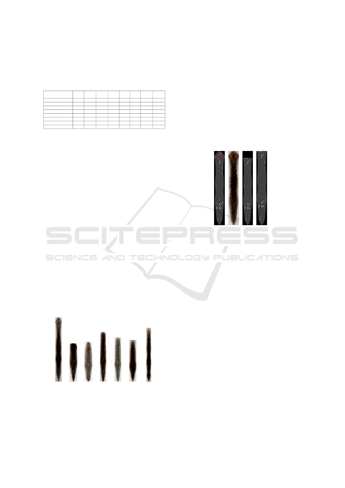
8.4 Regenerating Planaria

The “Regeneration” dataset consists of 579 images

capturing 20 planarians in the process of regeneration

after cutting off the head. Images were taken on the

ﬁrst, second, third, fourth, sixth and tenth days af-

ter decapitation, and images of whole planarians be-

fore decapitation are considered as a training sam-

ple. Also, 392 images of severed heads and organisms

evolved from them were obtained, but since they have

a small length and a small number of spots, they do

not ﬁt into the proposed model and their analysis was

left for further research. The process of regeneration

of a single planarian is shown in Fig. 9 and demon-

strates a very unpredictable shape change during the

process. It can be noted that the planarian as a whole

tends to restore its proportions, but the new spots that

have appeared in the head region do not coincide with

the old ones.

Day 0 Day 1 Day 2 Day 3 Day 4 Day 6 Day 10

Figure 9: Regeneration of planaria after cutting off the head.

To simulate the decapitation, eyes in the images

from the training sample were identiﬁed, and an as-

sumed cutting line was drawn at a level of 20 pixels

below eye level (Fig. 10ab). Further, the part of the

texture lying below this line was used for spot extrac-

tion (Fig. 10c) and the resulting pattern was stretched

in height (Fig. 10d). Such images were compared

with standards, which were considered to be the im-

ages of whole planarians before decapitation. As the

predicted cutting line may differ from the actual, the

stretching was carried out in the range from 80% to

120% of the texture height of a full planarian. The ﬁ-

nal quality of the classiﬁcation was 72.84%, the mis-

takes are explained by the instability of the planarian

morphology after decapitation and the need to predict

the dissection line.

(a) (b) (c) (d)

Figure 10: Processing the planarian after decapitation.

9 CONCLUSION

This study shows the fundamental possibility of iden-

tifying individual planarian ﬂatworms and makes it

possible to supplement observations of groups of indi-

viduals in biological experiments by tracking individ-

ual characteristics of development and regeneration.

The problems of detecting and segmentation of an

individual planarian in the image, approximating its

shape with a fat curve based on the medial represen-

tation and extracting the texture of the planarian in the

form of a rectangle of standard size are solved. It was

shown that the texture of a planarian is described with

sufﬁcient completeness by a set and arrangement of

light spots, which, on the one hand, are quite steadily

different between individuals, and, on the other hand,

are stable enough to persist for a rather long period of

time associated with the experiment. As directions for

further work, we can specify the processing of images

containing several animals and prediction

Identiﬁcation of Planarian Individuals by Spot Patterns in Texture

ACKNOWLEDGEMENTS

The work was funded by Russian Foundation of Basic

Research grant No. 20-01-00664.

REFERENCES

Apyari, V., Tiras, K., Nefedova, S., and Gorbunova, M.

(2021). Non-invasive in vivo spectroscopy using a

monitor calibrator: A case of planarian feeding and di-

gestion statuses. Microchemical Journal, 166:106255.

Bagu

a, J. (2012). The planarian neoblast: The rambling

history of its origin and some current black boxes.

The International Journal of Developmental Biology,

56:19–37.

Barber, B., K

uhn, D., Lo, A., Osthus, D., and Taylor, A.

(2017). Clique decompositions of multipartite graphs

and completion of latin squares. Journal of Combina-

torial Theory, Series A, 151:146–201.

Bay, H., Ess, A., Tuytelaars, T., and Gool, L. V. (2008).

Speeded-up robust features (surf). Computer Vision

and Image Understanding, 110(3):346–359. Similar-

ity Matching in Computer Vision and Multimedia.

Clapham, M., Miller, E., Nguyen, M., and Darimont, C.

(2020). Automated facial recognition for wildlife

that lack unique markings: A deep learning approach

for brown bears. Ecology and Evolution, 10:12883–

12892.

Dawande, M., Keskinocak, P., Swaminathan, J. M., and

Tayur, S. (2001). On bipartite and multipartite clique

problems. Journal of Algorithms, 41(2):388–403.

Duyck, J., Finn, C., Hutcheon, A., Vera, P., Salas, J., and

Ravela, S. (2015). Sloop: A pattern retrieval engine

for individual animal identiﬁcation. Pattern Recogni-

tion, 48(4):1059–1073.

Elliott, S. A. and Alvarado, A. S. (2013). The history and

enduring contributions of planarians to the study of

animal regeneration. Wiley Interdisciplinary Reviews:

Developmental Biology, 2:301–326.

Flygare, S., Campbell, M., Ross, R. M., Moore, B., and

Yandell, M. (2013). ImagePlane: An automated im-

age analysis pipeline for high-throughput screens us-

ing the planarian Schmidtea mediterranea. Journal of

Computational Biology, 20(8):583–592.

Freytag, A., Rodner, E., Simon, M., Loos, A., K

uhl, H.,

and Denzler, J. (2016). Chimpanzee faces in the wild:

Log-euclidean cnns for predicting identities and at-

tributes of primates. volume 9796, pages 51–63.

Fritsch, F. N. and Carlson, R. E. (1980). Monotone piece-

wise cubic interpolation. SIAM Journal on Numerical

Analysis, 17(2):238–246.

Hughes, B. and Burghardt, T. (2017). Automated visual ﬁn

identiﬁcation of individual great white sharks. Int. J.

Comput. Vis., 122(3):542–557.

Karami, A., Tebyaniyan, H., Gooadrzi, V., and Shiri, S.

(2015). Planarians: an in vivo model for regenera-

tive medicine. International Journal of Stem Cells,

8:128–133.

Lahiri, M., Tantipathananandh, C., Warungu, R., Ruben-

stein, D. I., and Berger-Wolf, T. Y. (2011). Biometric

animal databases from ﬁeld photographs: Identiﬁca-

tion of individual zebra in the wild. ICMR ’11, New

York, NY, USA. Association for Computing Machin-

ery.

Lee, V., Ruan, N., Jin, R., and Aggarwal, C. (2010). A

Survey of Algorithms for Dense Subgraph Discovery,

pages 303–336.

Liu, C., Zhang, R., and Guo, L. (2019). Part-pose guided

amur tiger re-identiﬁcation. In 2019 IEEE/CVF In-

ternational Conference on Computer Vision Workshop

(ICCVW), pages 315–322.

Lu, X., Wang, Y., Fung, S., and Qing, X. (2021). I-nema: A

biological image dataset for nematode recognition.

Mestetskiy, L. (2000). Fat curves and representation of pla-

nar ﬁgures. Computers & Graphics, 24:9–21.

Mestetskiy, L. and Semenov, A. (2008). Binary image

skeleton — continuous approach. In Proceedings

of the Third International Conference on Computer

Vision Theory and Applications - Volume 1: VIS-

APP, (VISIGRAPP 2008), pages 251–258. INSTICC,

SciTePress.

Myronenko, A. and Song, X. (2010). Point set registra-

tion: Coherent point drift. IEEE Transactions on Pat-

tern Analysis and Machine Intelligence, 32(12):2262–

2275.

Peiris, T., Hoyer, K., and Oviedo, N. (2014). Innate im-

mune system and tissue regeneration in planarians:

An area ripe for exploration. Seminars in Immunol-

ogy, 26:295–302.

Peng, H., Long, F., Liu, X., Kim, S. K., and Myers, E. W.

(2007). Straightening caenorhabditis elegans images.

Bioinformatics, 24(2):234–242.

Qu, L. and Peng, H. (2010). A principal skeleton algorithm

for standardizing confocal images of fruit ﬂy nervous

systems. Bioinformatics, 26(8):1091–1097.

Rao, K. K., Grabow, L. C., Mu

noz-P

erez, J. P., Alarc

on-

Ruales, D., and Azevedo, R. B. R. (2021). Sea turtle

facial recognition using map graphs of scales. bioRxiv.

Sheimann, I. M. and Sakharova, N. (1974). On a peculiarity

of planarian digestion. Comparative biochemistry and

physiology, 48:601–7.

Tiras, K., Mestetskiy, L., Nefedova, S., and Lomov, N.

(2021). Registration of regeneration in planarians

from photographic images. Journal of Biomedical

Photonics & Engineering.

Tiras, K., Petrova, O., Myakisheva, S., Deev, A., and

Aslanidi, K. (2015). Minimizing of morphometric

errors in planarian regeneration. Fundamental Re-

search, 2:128–133.

Tiras, K. P., Nefedova, S., Novikov, K., Emelyanenko, V.,

and Balmashov, S. (2018). In vivo methods of control

of phago- and pinocytosis on the model of planarian

digestion. In Proceedings of the International Con-

ference ”Situational Centers and Class 4i Informa-

tion and Analytical Systems for Monitoring and Secu-

rity Tasks” (SCVRT2018), volume 48, pages 346–359.

Moscow-Protvino.

VISAPP 2022 - 17th International Conference on Computer Vision Theory and Applications