Monocular Estimation of Translation, Pose and 3D Shape on Detected

Objects using a Convolutional Autoencoder

Ivar Persson

, Martin Ahrnbom

and Mikael Nilsson

Centre for Mathematical Sciences, Lund University, Sweden

{ﬁrst name.second name}@math.lth.se

Keywords:

Autoencoder, 6DoF-positioning, Trafﬁc Surveillance, Autonomous Vehicles, 6DoF Pose Estimation.

Abstract:

This paper present a 6DoF-positioning method and shape estimation method for cars from monocular images.

We pre-learn principal components, using Principal Component Analysis (PCA), from the shape of cars and

use a learnt encoder-decoder structure in order to position the cars and create binary masks of each cam-

era instance. The proposed method is tailored towards usefulness for autonomous driving and trafﬁc safety

surveillance. The work introduces a novel encoder-decoder framework for this purpose, thus expanding and

extending state-of-the-art models for the task. Quantitative and qualitative analysis is performed on the Apol-

loscape dataset, showing promising results, in particular regarding rotations and segmentation masks.

1 INTRODUCTION

In order to safely and reliably run autonomous cars,

or to have an automatic trafﬁc surveillance system, it

is necessary to detect and estimate position and rota-

tion of cars, just as a human driver or operator does

on a daily basis. The functionality and superiority of

using deep neural networks rather than traditional fea-

ture based methods to detect and classify objects, such

as cars, has been shown multiple times (Krizhevsky

et al., 2012; Fang et al., 2015). Traditionally you

would need two or more cameras to gain proper depth

information through triangulation, however, in recent

times this requirement has been avoided, for example

by using depth sensors (Li et al., 2020) or by using

neural networks (Chen et al., 2016; Liu et al., 2020;

Tatarchenko et al., 2016).

In this paper we present a method to estimate posi-

tion and rotation of cars in an urban environment. We

will, from a single image create a binary mask for the

car and an estimation of the true world coordinates,

both 3D position and 3D rotation. This method will be

based on the Skinned Multi-Animal Linear (SMAL)

method, formulated and used by Zufﬁ et al. (Zufﬁ

et al., 2017).

Our contribution is to build on the work by

Liu et al. (Liu et al., 2020), where 3D bounding boxes

https://orcid.org/0000-0003-4958-3043

https://orcid.org/0000-0001-9010-7175

https://orcid.org/0000-0003-1712-8345

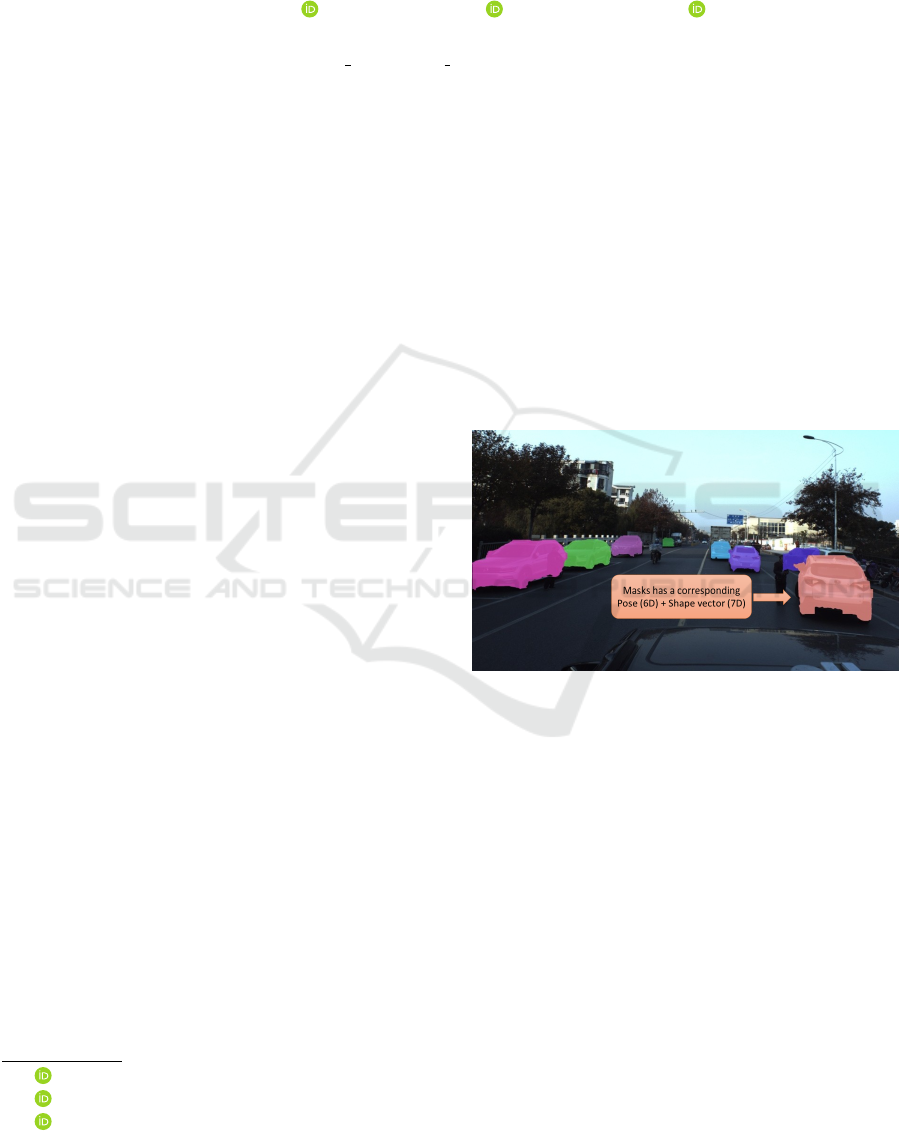
Figure 1: Intended result, of the Encoder-Decoder solution

presented in this paper. All masks are sorted by z-distance

to show the correct mask, formed from pose and shape vec-

tors, where different cars overlap.

are calculated for cars. We will in the same man-

ner detect cars, however, we will instead calculate

a per-pixel binary mask segmentation of the car, by

using keypoints and a learnt decoder. The segmen-

tation mask will be based on the SMAL method by

Zufﬁ et al. (Zufﬁ et al., 2017), where a shape model

is ﬁtted to a pre-learnt space of principal components,

using Principal Component Analysis (PCA), from the

keypoints. These results are of interest as a camera

mounted on a car can then detect and position cars

from a single image, rather than two. Apart from an

Automated Driving context this can also be used in

Trafﬁc Monitoring to e.g. monitor busy intersections.

The idea is that this method can be relatively easily

expanded, given training data, to cover not only cars

but also other road users, such as lorries, bicycles and

390

Persson, I., Ahrnbom, M. and Nilsson, M.

Monocular Estimation of Translation, Pose and 3D Shape on Detected Objects using a Convolutional Autoencoder.

DOI: 10.5220/0010826600003124

In Proceedings of the 17th International Joint Conference on Computer Vision, Imaging and Computer Graphics Theory and Applications (VISIGRAPP 2022) - Volume 5: VISAPP, pages

390-396

ISBN: 978-989-758-555-5; ISSN: 2184-4321

possibly pedestrians, but then maybe with some mod-

elling modiﬁcations to better cope with more non-

rigidity.

The training and validation is done with the Apol-

loscape dataset, by Song et al. (Song et al., 2019).

This dataset is an extensive dataset spanning multi-

ple problems in autonomous driving, where the car

instance part will be used in this paper. Over 4000

images for training, containing 47573 annotated cars,

and 200 images for validation, containing 2403 anno-

tated cars. Each annotated car have been annotated

with semantic keypoints, along real-world spatial co-

ordinates relative to the camera and relative euler an-

gle rotation are provided.

2 RELATED WORK

Many previous advances in the ﬁeld of 3D reconstruc-

tion have been made. One of the key points of this

paper is to predict 3D translation of cars from a sin-

gle image. Earlier you would have needed specialised

sensors to get depth information or by using a stereo

camera pair, as Chen et al. (Chen et al., 2015) uses.

This technique is still useful and relevant, especially

in robotics (Grenzd

orffer et al., 2020). However, with

the introduction of Deep Neural Netowks (DNNs),

single image 3D detection and ﬁtting of 3D boxes on

the cars have been made possible (Mousavian et al.,

2017; Liu et al., 2020). Here (Mousavian et al., 2017)

uses the 2D bounding boxes from an object detec-

tor as input and creates a 3D box from this, with one

side of the bounding box denoting the front of the car.

Chabot et al. (Chabot et al., 2017) takes this idea one

step further by taking a 3D box and, with the help of

semantic keypoints, make a ﬁner segmentation mask.

One distinction between different 6DoF-

estimation systems is whether the implementation

is end-to-end (Zou et al., 2021; Kundu et al., 2018)

or if you use high-performance object detectors to

get bounding boxes and cropped images as input

to the system (Mousavian et al., 2017). We will

use the latter and generate results similar to the

work by Mousavian et al. (Mousavian et al., 2017)

and Chabot et al. (Chabot et al., 2017), but with a

closer ﬁt to the shape of cars. In order to achieve

this we will use robust shape models, pre-learnt

and calculated similarly to the SMAL method pre-

sented by Zufﬁ et al. (Zufﬁ et al., 2017). A similar

approach to what we do can be found in the work

by Kundu et al. (Kundu et al., 2018). The main

difference is that they use a differentiable render-and-

compare operation, while we reduce the complexity

of the solution by using a learnt decoder network.

3 METHOD

The idea behind the method is to create an average car

that can be modiﬁed to better ﬁt different car models.

We use the detailed car models in the Apolloscape

dataset, by Song et al. (Song et al., 2019), as a basis

together with the semantically useful keypoints also

provided in the dataset. The keypoints are mapped

to each car model. With this mapping we have 66

semantic keypoints from 34 different car models.

Further on we make use of the results presented by

Zufﬁ et al. (Zufﬁ et al., 2017) who use average shape

of four-legged animals. Here, we do not need to think

about bending of joints as the cars are rigid bodies.

3.1 SMAL

Zufﬁ et al. presents the SMAL model in (Zufﬁ et al.,

2017) where they describe a function to estimate

shapes and poses of animals. Animals’ ﬂexibility is

also addressed in this model, however, since cars are

inﬂexible we can simplify the equations to

i,p

= m + Dθ

. (1)

Here m is the template, or mean, of a car, θ

is the

vector of parameters describing car i and D is a learnt

PCA-space for all available car models. This equals

i,p

, which is car i parameterized. Both the mean, m

and the PCA-space D will be discussed further in 3.2.

Zufﬁ et al. presented their model as:

= t

+ m

p,i

+ B

s,i

+ B

p,i

, (2)

where p

is part i of the animal. t

is a template, m

p,i

the average pose displacements, B

s,i

is a matrix with

columns containing basis of shape displacements and

p,i

is a matrix with the basis of pose displacements.

This equation is formulated for dividing the ani-

mal in several pieces where each piece can be bent

and moved independently (but still being connected

with each other). We, however, have rigid cars and

we do not divide the car into several pieces, but keep

it as one.

Therefore, we can ignore the terms B

p,i

and m

p,i

as they will be zero for rigid objects. By simplifying

notation as t

= m, B

s,i

= D and also renaming s

to θ

we have then simpliﬁed Equation 2 into 1.

The PCA-space, D, in Equation 1, allows us to es-

timate shapes of cars robustly while only having to es-

timate the elements of θ

in the Encoder. The SMAL

method is then a matter of minimising the error

E(θ

) = (C

−C

i,p

)

, (3)

Monocular Estimation of Translation, Pose and 3D Shape on Detected Objects using a Convolutional Autoencoder

391

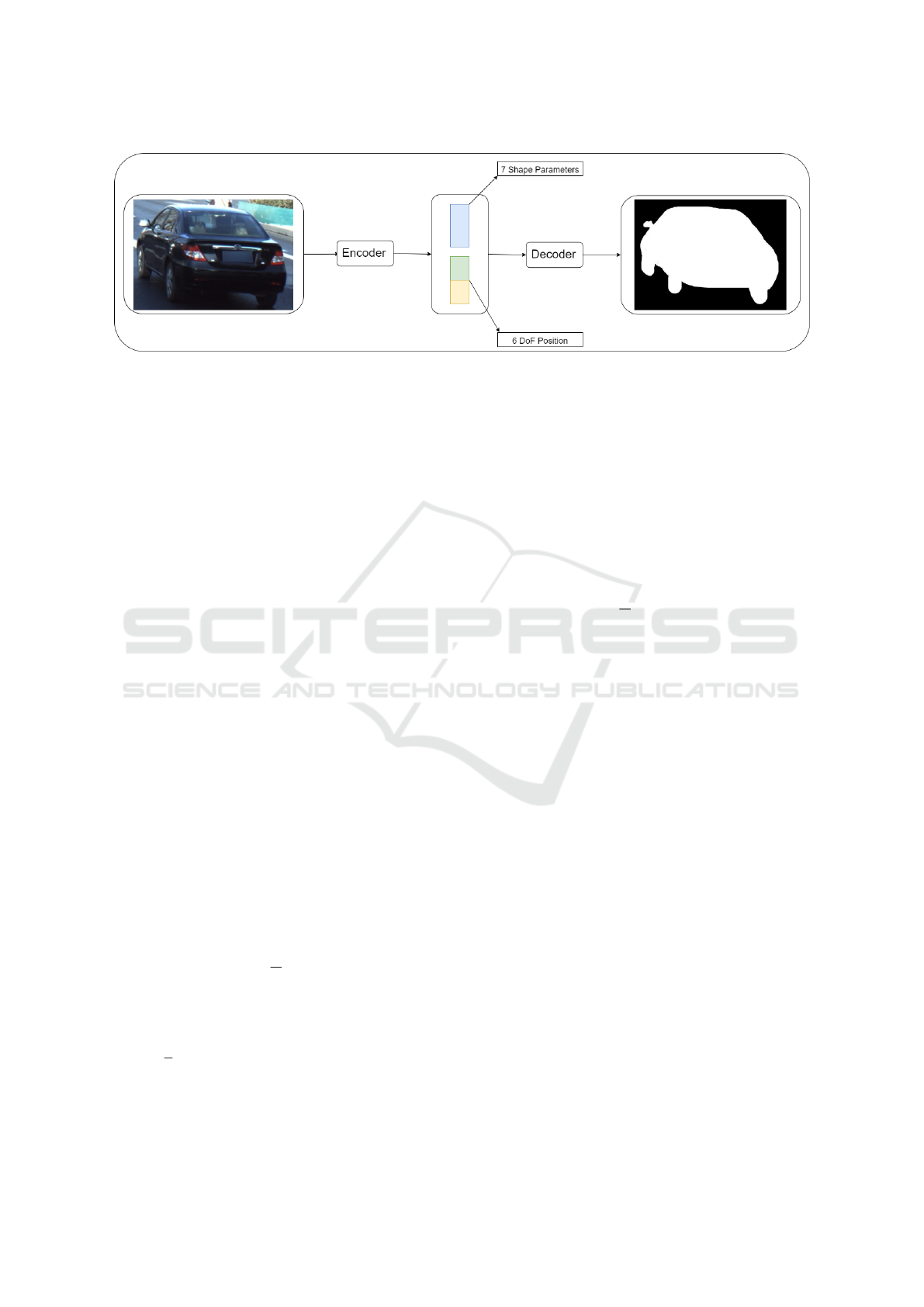
Figure 2: Overview of the workﬂow of the system. Cars are cropped out of the images, after detections by Detectron2 (Wu

et al., 2019). The encoder get information about the pixel-location of the crop and then reduces the crop information and the

cropped car to 14 elements. Six elements describe the translation and rotation of the car, while the remaining seven are the

shape parameters θ

in equation 6. The (x, y, z) distance of the car from the camera can be obtained here before the encoded

information is fed into the decoder network. The decoder then restores the position of the crop and creates a binary mask of

the car.

where C

is the true positions of the keypoints of car

i and C

i,p

is the estimations from Equation 1, depen-

dent on θ

. As mentioned in (Zufﬁ et al., 2017), the

SMAL model is robust enough that it can generalise

to shapes, in their context of four-footed animals, un-

seen before in training. This method should there-

fore be able to generalise to car models unseen before,

which makes this method desirable since it would be

impossible to model all car designs in the world.

3.2 Generalised Procrustes Analysis

The template shape from the description of SMAL

is calculated using Generalised Procrustes Analysis.

This method allows us to compute an average shape

that can be altered with additional low dimension in-

formation. We follow the description presented by

Stegmann and Gomez (Stegmann and Gomez, 2002).

We choose a shape as the mean shape and align all

other shapes to this, e.g. we choose x

, where x

is the

vector of car i. Normally we would need to translate,

rotate and scale all feature points, however, since all

cars, created from the data by Song et al. (Song et al.,

2019), are rotated equally and of the same size, only a

slight translation is needed. To translate we calculate

the mean

m =

∑

i=0

, (4)

and translate the cars x

= x

− m. We have N as

the number of cars. We calculate the average of all

points for all cars, thus creating a new template shape,

(k) =

∑

i=0

(k), where x

(t) is the template shape

at keypoint k. We continue to align the shapes x

to the template shape x

and calculate a new mean

m. When m converges we have found our template

shape x

. Typically this only takes a couple of itera-

tions (Stegmann and Gomez, 2002).

Next, we calculate a difference between all shapes

and the template dx

= x

− x

. By calculating the

outer product of dx

with it self we can calculate a

correlation matrix

D =

∑

i=0

. (5)

We calculate the eigenvalues and corresponding

eigenvectors to D and analyse the magnitudes of the

eigenvalues. We take the corresponding eigenvectors

to the greatest eigenvalues and form a new matrix

, where L is the number of eigenvectors used. We

can then approximate each car by x

= x

+ D

, for

some θ

unique to each car and using all eigenvec-

tors of D

. By reducing the number of eigenvectors

we can simplify our model, making it more robust to

noise in the eigenvectors and also reduce the amount

of data stored. The number of eigenvectors was exper-

imentally decided on upon observing the eigenvalues

and ﬁnding that a suitable cutoff seemed to be using

seven eigenvectors (L = 7). These seven eigenvec-

tors, stacked column-wise, are denoted by the matrix

. The best approximation to each car is then given

= D

, (6)

where each θ

then can be used in Equation 1. This

method can be seen as a special case of Principal

Component Analysis (PCA).

VISAPP 2022 - 17th International Conference on Computer Vision Theory and Applications

392

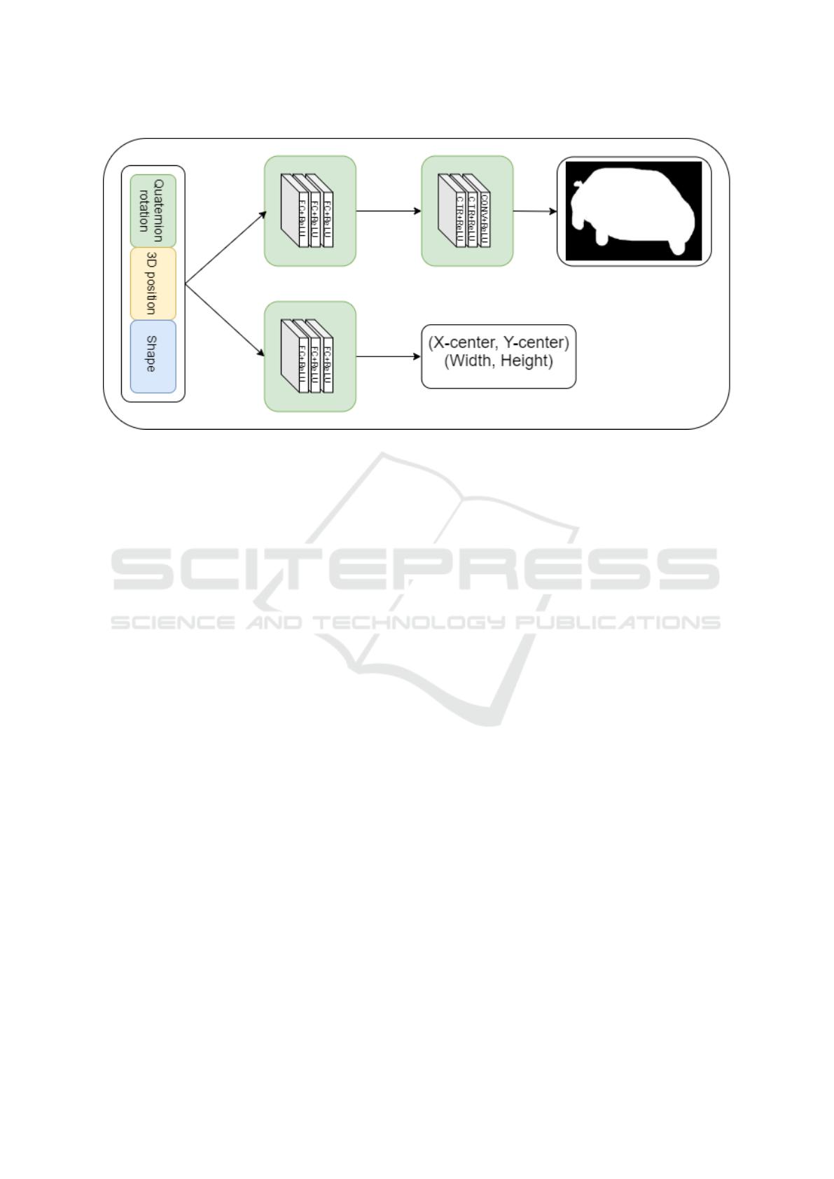
Figure 3: Workﬂow of the decoder network. The input is a 14 element pose-and-shape vector, consisting of seven shape

parameters and six pose parameters. The network is divided in two parts, where the mask network creates a mask, given the

pose rotation of the car, while the crop network creates pixel values (x

, y

) of the centre of the crop as well as height and

width of the crop. The exact structure of the mask and crop part of the network can be seen in Table 1). These two pixel pairs

are then used to insert the mask in the 2d-space of the image.

4 AUTOENCODER

The structure to solve this problem is by using a

encoder-decoder network and using a similar training

regime as (Tan et al., 2017) use. We use the encoder

to ﬁnd pose and shape parameters, and as a second

step use a decoder network to create binary masks of

all cars present.

The seven element shape vector, θ

, is calculated

from equation 6 and concatenated with the pose infor-

mation, four coordinates of rotation (quartenions) and

three coordinates of translation, to form a 14 element

vector. This vector is the output from the encoder net-

work and also the input to the decoder network.

4.1 Pre-processing

All data points were normalised to a range suitable for

their purpose. The centre point of the crop informa-

tion as well as the width and height were altered to be

in the range [−1, 1], while the binary masks were al-

ready binary. The 3D-position in the encoded vector

was also normalised with the largest (absolute) value

in the dataset in order to ﬁt the output of a tanh acti-

vation function.

4.2 Encoder

The encoder takes input in the form of cropped RGB-

images, reshaped to (256, 256, 3). These crops are

detected using Detectron2 (Wu et al., 2019), before

being used as inputs to the encoder. Along the im-

age there is also information regarding what parts in

the image the detection was made. This is fed as a

vector of six integers describing (x, y) center point,

width and height of the crop but also the area and as-

pect ratio of the crop. The output is a vector of 14

elements of which seven are the shape-parameters of

the car, four are the quaternion rotation and three are

the translation. The network structure is described

in Figure 4. The base of the network is a pre-learnt

ResNet50 feeding fully connected layers.

4.2.1 Loss Functions

The loss function is a standard mean squared error for

the shape and the 3D-position has a mean absolute

error. The quaternion rotation vector is normalised

before a scalar product and arccos is the loss for the

rotation. We get

rot

= acos(< Q

est

, Q

>), (7)

where L

rot

is the loss in degrees and Q

est

and Q

are

the estimated quaternion and the ground truth quater-

nion. Since |Q

est

| = |Q

| = 1 we get the arc cosine of

Monocular Estimation of Translation, Pose and 3D Shape on Detected Objects using a Convolutional Autoencoder

393

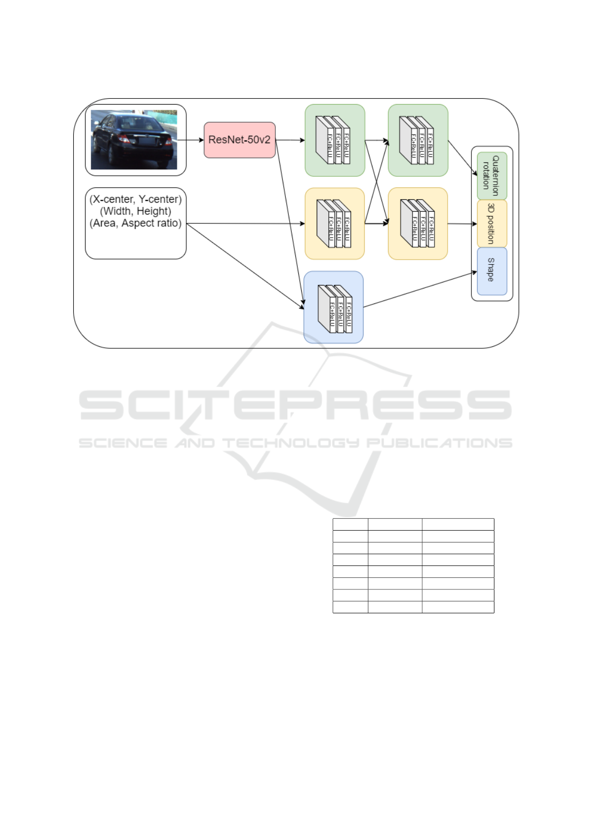
Figure 4: Workﬂow of the encoder network. The input is the cropped image of the car and crop information values: (x, y)

centre points, width, height and also area and aspect ratio. The image is fed through a ResNet-50 pre-trained network, where

the head is removed. The output from the ResNet-50 network as well as the crop information is fed through a series of fully

connected layers as shown in the image, the exact structure is described in 4.2.2.

the cosine of the angle between the two vectors, i.e.

the angle between the two quartenion vectors. This

is the same metric used in the original Apolloscape

challenge.

4.2.2 Structure

Each coloured square in Figure 4 is comprised of

three fully-connected layers, all with 512 units, with

Rectiﬁed Linear Unit (ReLU) activation and subse-

quent dropout of 20%. The idea is that both the

quaternion rotation and the 3D position needs the in-

formation from both the cropped image as well as the

crop information and should therefore share this in-

formation.

4.3 Decoder

The decoder network uses the output from the en-

coder, the 14 element vector, as input. Using a similar

network structure as (Tan et al., 2017), we calculate a

binary mask of the car given the encoded values, in-

cluding the shape parameters. We do, however, in par-

allel also calculate the position and size of where the

binary mask should be located in the recreated image.

This can be seen in Figure 3, where the layers of mask

calculation and the layers of the crop positioning are

done in parallel without any shared weights. These

two tasks were considered such that there would be no

beneﬁts in combining layers such as is done in the en-

coder. The decoder network uses the calculated crop

information to reshape and place the calculated mask

in an image with the same dimensions as the original

image that was fed into Detectron2. The entire struc-

ture in detail is shown in Table 1 and 2.

Table 1: Structure of the Decoder network for the mask.

This corresponds to the top row in Figure 3.

Layer Function Size

Input 14

1 Dense 256

2 Dense 500

3 Dense 810

- Reshape 9 × 9 × 10

4 Conv2DTr 63 × 63 × 384

5 Conv2D 59 × 59 × 1

5 RESULTS

The evaluation of the results can be split up in the en-

tire Encoder-Decoder structure as well as the Encoder

and Decoder separately. For this paper we only con-

sider the Encoder and the Decoder separately. The

Encoder by itself is interesting since we can obtain

VISAPP 2022 - 17th International Conference on Computer Vision Theory and Applications

394

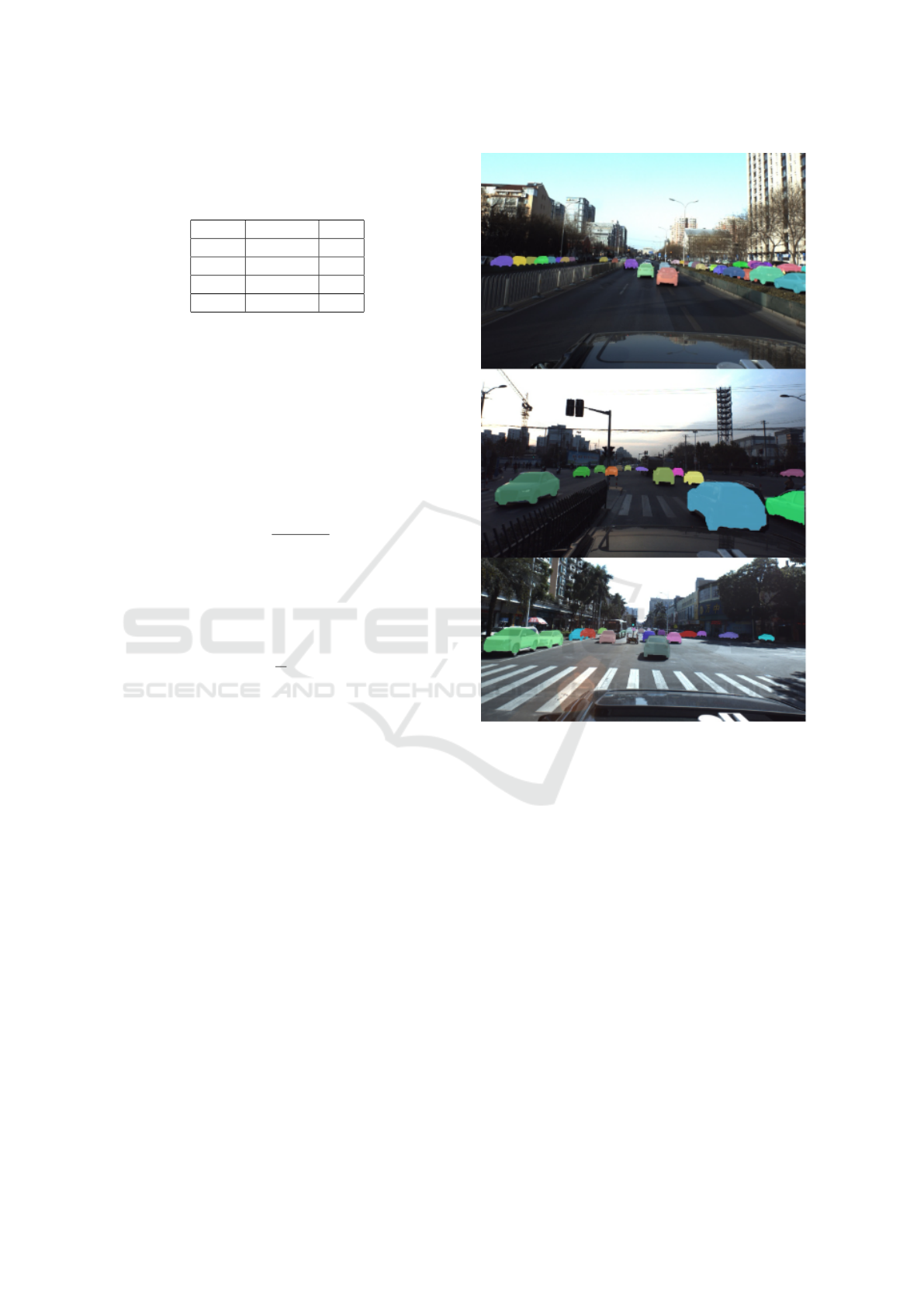
Table 2: Structure of the Decoder network for the crop in-

formation, i.e. the second row in Figure 3. The output of

four values are the (x, y) centre points and also the width

and height of the crop.

Layer Function Size

Input 14

1 Dense 512

2 Dense 256

3 Dense 4

the real-world position and rotation of the detected

cars. By analysing the Decoder by itself will yield

interesting data on how well the decoder can trans-

form real-world positions to pixel coordinates in the

images. Exploring the full Encoder-Decoder structure

on data with only segmentation and no 3D annotation,

is considered a future work direction.

The performance of the Decoder for each sample

is done by the Intersection over Union (IoU), calcu-

lated as

IoU

∩ M

∪ M

, (8)

where M

is the ground truth mask of sample i and

is the estimated mask from sample i, giving a

score between 0 and 1 for each sample in the dataset.

A mean IoU,

mIoU =

∑

IoU

, (9)

over the entire dataset is presented as the average

score in Table 4. The entire Encoder-Decoder struc-

ture can then also be evaluated using the same met-

ric. The resulting 3D position and quaternion rota-

tion from the Encoder can be evaluated with the same

metrics used in the original Apolloscape competition

(Apolloscape, 2021). The translation error is a sim-

ple L2-norm and the rotation error is the same as the

loss function, used in the Encoder training and pre-

sented in Equation 7. The results are presented in

Table 3 where the percentage of cars with an error

smaller than a threshold are calculated. Some results

are visualised in Figure 5.

In Table 4 we present the results from the Decoder

in a manner very similar to what they did in the Apol-

loscape competition (Apolloscape, 2021), however it

can not be compared directly as we only examine the

shape conforming ability in the current view while in

the Apolloscape competition multiple views were ex-

amined.

Figure 5: Three randomly picked images from the valida-

tion set and their binary masks as overlay. Note that the im-

ages are cropped in order to display the results more clearly.

Best viewed in colour.

6 CONCLUSIONS

In this work a novel encoder-decoder framework is in-

troduced, with the focus on estimating translation, ro-

tation and shape of cars from a monocular view. The

aim is to use this network in new situations with car

models unseen in training. We have only worked with

cars in this paper, but the method could be generalised

for lorries, motorcycles, bicycles and other rigid ob-

jects directly, while some additional shape modelling

of non-rigid objects are likely warranted. Results on

the Apolloscape dataset highlight the current perfor-

mance of the system. Evaluation shows promising

performance in particular regarding the rotation and

segmentation masks.

Monocular Estimation of Translation, Pose and 3D Shape on Detected Objects using a Convolutional Autoencoder

395

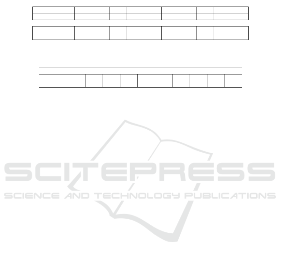
Table 3: Results on the estimation of rotation and translation. Each estimation was evaluated and compared against a set of

thresholds. Results given on the validation dataset from Apolloscape.

Total: 2245 images in validation set

Rotation - 18.0

average error

Error (degrees) 5

% of cars 73.3 80.7 82.8 85.5 86.2 86.1 86.7 87.0 87.2 87.5

Translation - 4.8m average error

Error (meters) 0.1 0.4 0.7 1.0 1.3 1.6 1.9 2.2 2.5 2.8

% of cars 0.09 2.6 8.0 14.4 21.7 27.1 33.2 38.4 43.5 48.0

Table 4: Results on the quality of the binary mask, where the score of each mask was compared with a set of thresholds.

Results given on the validation dataset from Apolloscape.

Total: 2403 images in validation set

Average IoU (Decoder) - 88%

IoU 0.95 0.9 0.85 0.8 0.75 0.7 0.65 0.60 0.55 0.5

% of cars 14.9 57.8 80.8 90.4 94.3 96.4 97.8 98.7 99.3 99.5

REFERENCES

Apolloscape (2021). Apolloscape, car instance - metric for-

mula. http://apolloscape.auto/car instance.html.

Chabot, F., Chaouch, M., Rabarisoa, J., Teuli

ere, C., and

Chateau, T. (2017). Deep manta: A coarse-to-ﬁne

many-task network for joint 2d and 3d vehicle analy-

sis from monocular image. In 2017 IEEE Conference

on Computer Vision and Pattern Recognition (CVPR),

pages 1827–1836.

Chen, X., Kundu, K., Zhang, Z., Ma, H., Fidler, S., and

Urtasun, R. (2016). Monocular 3d object detection

for autonomous driving. In 2016 IEEE Conference

on Computer Vision and Pattern Recognition (CVPR),

pages 2147–2156.

Chen, X., Kundu, K., Zhu, Y., Berneshawi, A. G., Ma, H.,

Fidler, S., and Urtasun, R. (2015). 3d object propos-

als for accurate object class detection. In Cortes, C.,

Lawrence, N., Lee, D., Sugiyama, M., and Garnett,

R., editors, Advances in Neural Information Process-

ing Systems, volume 28, pages 424–432.

Fang, H., Gupta, S., Iandola, F., Srivastava, R., Deng, L.,

Dollar, P., Gao, J., He, X., Mitchell, M., Platt, J., Zit-

nick, L., and Zweig, G. (2015). From captions to vi-

sual concepts and back. In The proceedings of CVPR.

IEEE - Institute of Electrical and Electronics Engi-

neers.

Grenzd

orffer, T., G

unther, M., and Hertzberg, J. (2020).

Ycb-m: A multi-camera rgb-d dataset for object

recognition and 6dof pose estimation. In 2020 IEEE

International Conference on Robotics and Automation

(ICRA), pages 3650–3656.

Krizhevsky, A., Sutskever, I., and Hinton, G. (2012). Im-

agenet classiﬁcation with deep convolutional neural

networks. In NIPS’12: Proceedings of the 25th Inter-

national Conference on Neural Information Process-

ing Systems, pages 1097–1105.

Kundu, A., Li, Y., and Rehg, J. M. (2018). 3d-rcnn:

Instance-level 3d object reconstruction via render-

and-compare. In 2018 IEEE/CVF Conference on

Computer Vision and Pattern Recognition, pages

3559–3568.

Li, Z., Yu, T., Pan, C., Zheng, Z., and Liu, Y. (2020). Robust

3d self-portraits in seconds. In 2020 IEEE/CVF Con-

ference on Computer Vision and Pattern Recognition

(CVPR), pages 1344–1353.

Liu, Z., Wu, Z., and T

oth, R. (2020). Smoke: Single-stage

monocular 3d object detection via keypoint estima-

tion. In 2020 IEEE/CVF Conference on Computer

Vision and Pattern Recognition Workshops (CVPRW),

pages 4289–4298.

Mousavian, A., Anguelov, D., Flynn, J., and Ko

seck

a, J.

(2017). 3d bounding box estimation using deep learn-

ing and geometry. In 2017 IEEE Conference on Com-

puter Vision and Pattern Recognition (CVPR), pages

5632–5640.

Song, X., Wang, P., Zhou, D., Zhu, R., Guan, C., Dai, Y.,

Su, H., Li, H., and Yang, R. (2019). Apollocar3d:

A large 3d car instance understanding benchmark for

autonomous driving. In 2019 IEEE/CVF Conference

on Computer Vision and Pattern Recognition (CVPR),

pages 5447–5457.

Stegmann, M. B. and Gomez, D. D. (2002). A brief intro-

duction to statistical shape analysis.

Tan, V., Budvytis, I., and Cipolla, R. (2017). Indirect deep

structured learning for 3d human body shape and pose

prediction. In 2017 British Machine Vision Confer-

ence (BMVC).

Tatarchenko, M., Dosovitskiy, A., and Brox, T. (2016).

Multi-view 3d models from single images with a con-

volutional network. In European Conference on Com-

puter Vision, ECCV 2016, pages 322–337.

Wu, Y., Kirillov, A., Massa, F., Lo, W.-Y.,

and Girshick, R. (2019). Detectron2.

https://github.com/facebookresearch/detectron2.

Zou, W., Wu, D., Tian, S., Xiang, C., Li, X., and Zhang, L.

(2021). End-to-end 6dof pose estimation from monoc-

ular rgb images. IEEE Transactions on Consumer

Electronics, 67(1):87–96.

Zufﬁ, S., Kanazawa, A., Jacobs, D. W., and Black, M. J.

(2017). 3d menagerie: Modeling the 3d shape and

pose of animals. In 2017 IEEE Conference on Com-

puter Vision and Pattern Recognition (CVPR), pages

5524–5532.

VISAPP 2022 - 17th International Conference on Computer Vision Theory and Applications

396