Vision Transformers for Brain Tumor Classiﬁcation

Eliott Simon and Alexia Briassouli

Department of Data Science and Knowledge Engineering, Maastricht University, The Netherlands

Keywords:

Brain Tumor Classiﬁcation, Deep Learning, Vision Transformer, Convolutional Neural Network.

Abstract:

With the increasing amount of data gathered by healthcare providers, interest has been growing in Machine

Learning, and more speciﬁcally in Deep Learning. Medical applications of machine learning range from

the prediction of medical events, to computer-aided detection, diagnosis, and classiﬁcation. This paper will

investigate the application of State-of-the-Art (SoA) Deep Neural Networks in classifying brain tumors. We

distinguish between several types of brain tumors, which are typically diagnosed and classiﬁed by experts

using Magnetic Resonance Imaging (MRI). The most common benign tumors are gliomas and meningiomas,

however there exist many more which vary in size and location. Convolutional Neural Networks (CNN) are

the SoA deep learning technique for image processing tasks such as image segmentation and classiﬁcation.

However, a recently developed architecture for image classiﬁcation, namely Vision Transformers, have been

shown to outperform classical CNNs in efﬁciency, while requiring fewer computational resources. This work

introduces using only Transformer networks in brain tumor classiﬁcation for the ﬁrst time, and compares their

performance with CNNs. A signiﬁcant difference between the two models, tested in this manner, is the lack

of translational equivariance in Transformers, which the CNNs already have. Experiments for brain tumor

classiﬁcation on benchmark real-world datasets show they can achieve comparable or better performance,

despite using limited training data.

1 INTRODUCTION, RELATED

WORK

Brain tumors appear when there is an uncontrolled,

abnormal growth of cells in the central nervous sys-

tem. Although the cause of most brain tumors re-

mains unknown, experts can easily classify them in

different categories. Brain tumours are either benign

(non-cancerous), or malignant (cancerous) (Herholz,

2012). According to The Cancer Research UK, the

most common types of brain tumours are Glioma,

Meningioma, and Pituitary. Magnetic Resonance

Imaging (MRI) is a powerful non-invasive imaging

technology which allows to produce detailed anatom-

ical images of brain tumors. With the help of MRI

scans, an expert is able to determine the category of a

tumor, as well as its size and location (Scans, 2021).

With the advent of deep learning in medical imag-

ing applications, CNNs were introduced for brain tu-

mor classiﬁcation in several works, achieving good

accuracy (Hossain et al., 2019), (Badza and Barjak-

tarovic, 2020). Various CNNs were examined in

(Rehman et al., 2019), in combination with very ef-

https://orcid.org/0000-0002-0545-3215

ﬁcient data augmentation techniques, for brain tu-

mor classiﬁcation, achieving an accuracy of 98.69%

(Rehman et al., 2019) on a 2017 dataset. However,

rapid advances in the ﬁeld have led to the develop-

ment of better performing, context-aware networks,

such as Transformers, ﬁrst for Natural Language Pro-

cessing (NLP), extended to computer vision.

Vision Transformer (ViT) models are usually im-

plemented for image classiﬁcation or segmentation

tasks. For the sake of tumor diagnosis, ViT models

have only recently been examined, resulting in very

promising outcomes. For example, the TransBTS

(Wang et al., 2021) model allows to detect the pres-

ence of a brain tumor in a 3D MRI environment. The

model outperformed other 3D segmentation models,

reaching an accuracy of 90% (Wang et al., 2021).

Other models, such as TransMed (Dai et al., 2021),

which consists of a combination of Transformer and

CNN, have further improved the quality of tumor di-

agnosis. The reason for combining the two archi-

tectures is that most tumor classiﬁcation datasets are

small, while the efﬁciency of transformer networks

still highly depends on the amount of data used for

training (Dai et al., 2021).

Simon, E. and Briassouli, A.

Vision Transformers for Brain Tumor Classiﬁcation.

DOI: 10.5220/0010834300003123

In Proceedings of the 15th International Joint Conference on Biomedical Engineering Systems and Technologies (BIOSTEC 2022) - Volume 2: BIOIMAGING, pages 123-130

ISBN: 978-989-758-552-4; ISSN: 2184-4305

123

In this paper, we examine for the ﬁrst time the de-

tection and classiﬁcation of tumors from a recent MRI

Brain tumor dataset (MRI Kaggle dataset, 2020) us-

ing ViTs alone, that are trained from scratch. The

SoA on this dataset is based on CNNs, and attained an

accuracy of 95.40% (Badza and Barjaktarovic, 2020),

while ViT’s have not been applied to it. Speciﬁcally,

at the time of writing this paper, VIT’s alone had not

been applied to the problem of brain tumor detection

and classiﬁcation on related datasets, including the re-

cent only used here (MRI Kaggle dataset, 2020).

Unlike past works, our approach relies solely on

transformers, trained from scratch on this relatively

small dataset. We compare their performance to that

of a CNN, which we designed and trained for this

dataset, demonstrating that they outperform it as well.

Overall, ViT’s are demonstrated to perform very well,

despite lacking in inductive biases, translational in-

variance and equivariance that characterize CNNs,

while being trained from scratch on a relatively small

training dataset. This indicates that ViTs alone can be

used for tumor detection and classiﬁcation, but also -

indirectly - shows the role of spatial attention in ViT

vs. translational invariance that is present in CNNs.

Data augmentation was also examined, but shown to

require more computational resources, in order for

the augmented datasets to be appropriately leveraged,

as in (Rehman et al., 2019), leading us to conclude

its potential for improving results is possible when

higher computational resources are available.

This paper is structured as follows: Section 2 de-

scribes the dataset that is used for classiﬁcation, and a

binarized version we create for detection. The meth-

ods used are presented in Section 3, where a descrip-

tion of the general Transformer Network architecture

is given, followed by its application in Computer vi-

sion, known as Vision Transformers, and the CNN

used in this work for comparison. Experimental re-

sults are presented in Sections 4 and section 5 presents

our conclusions and future research directions.

2 DATASET

We consider a recent (2020) data set of Magnetic Res-

onance Imaging (MRI) annotated data, where each

image depicts either a type of brain tumor (one of

three types), or no tumor (MRI Kaggle dataset, 2020).

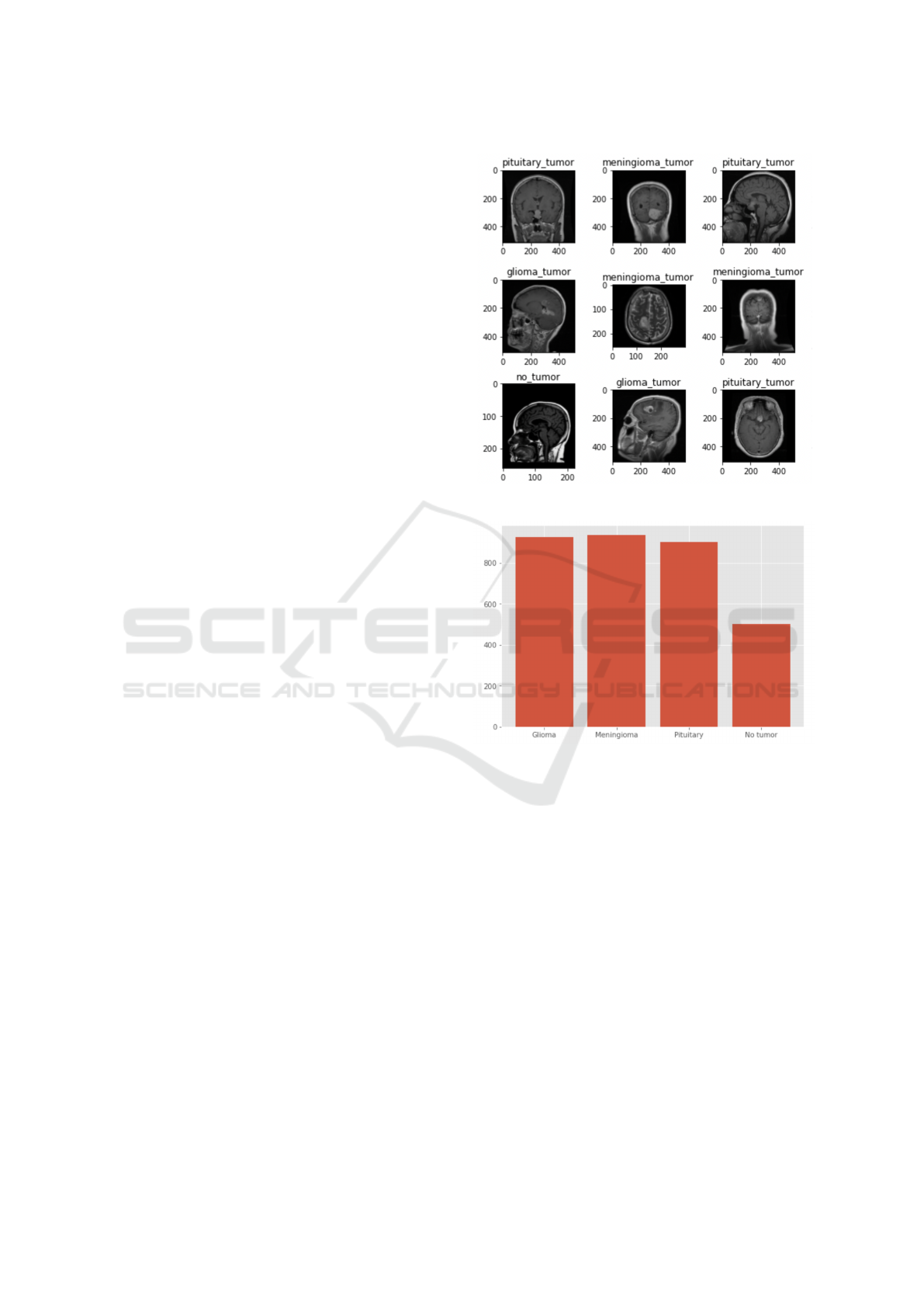
Some characteristic images from it are shown in

Fig. 1. Detecting and classifying these tumors is a

typical classiﬁcation problem, therefore a lot of data

is required in order to build a robust model (He et al.,

2016). A rule of thumb is that 1000 of images per

class is already enough (Warden, 2017).

Figure 1: Sample images from the benchmarking data set.

Figure 2: Number of images per each category.

Our testing dataset contains 100 images of glioma

tumors, 115 of meningioma tumors, 74 of pituitary

tumors and 105 with no tumor. Our training dataset

contains 826 images of glioma tumors, 822 of menin-

gioma tumors, 827 of pituitary tumors and 395 with

no tumor. The dataset does not contain any external

information about the patients, therefore its applica-

tion is restricted to image classiﬁcation. The distri-

bution of the data among the different classes is quite

balanced, with a lower amount of no tumor images

available for training, as shown in Fig. 2.

2.1 Binary Data Set

In order to examine the performance of ViT’s on the

detection problem, we ﬁrst consider the simpler prob-

lem of detecting the presence of a tumor versus no

tumor. To this end, we created a binary data set

from (MRI Kaggle dataset, 2020), which contains

BIOIMAGING 2022 - 9th International Conference on Bioimaging

124

Figure 3: Distribution of Binary Dataset.

only two classes. The idea is to merge the glioma,

meningioma, and pituitary into a single tumor-class.

The other class contains the images of a brain with

no brain tumor. The resulting binary dataset is quite

unbalanced, because the images with tumors have far

more data available for training (Fig. 3), however it is

expected to sufﬁce for the binary detection problem.

For both the binary and original data split, data

augmentation is a plausible approach to addressing

dataset imbalance and improving performance. For

our kind of data, data augmentation needs to be ap-

plied carefully so as to not modify informative pixel

values in the images, so we only tested different

kinds of image rotation. Our experiments showed

that, for this data, rotation did not improve results,

indicating that it did provide sufﬁcient variation in

the augmented training data, so we did not pursue it

further. Effective data augmentation would require

higher computational resources and extensive train-

ing, in order to sufﬁciently leverage the additional in-

formation in the augmented data and explore its effect

in depth, which is beyond the scope of this work.

3 METHODS

3.1 Transformer Network

Transformer Networks became the SoA technique for

many Natural Language Processing tasks, such as ma-

chine translation, or text summarization (Wang et al.,

2019). Similarly to Recurrent Neural Networks, the

input data must be sequential. However, the novel

transformer model uses parallelization, which consid-

erably reduces the training time.

The core of the model consists of an encoder-

decoder architecture (Vaswani et al., 2017). In Recur-

rent Neural Networks, the encoder generates an em-

bedding for each word, one at a time. However, each

instance of a word depends on the previously embed-

ded words, which leads to very inefﬁcient results for

large texts (Cho et al., 2014). In transformer mod-

els this issue is surpassed, as the encoder of a trans-

former model captures the entire sequence and gen-

erates an embedding for each word simultaneously.

Each of these embeddings consists in a vector that

encapsulates the meaning of the word. Therefore,

similar words have closer numbers in their vectors

(Zichao and et al., 2016). Since similar words may

have different meanings, the model uses a positional

encoder, which provides some context, based on the

positions of the words in the sentence. Thereafter,

the embedding vectors that contain context about the

words are fed into the encoder block. The ﬁrst step

of this encoder block involves attention, which deter-

mines the most important parts of the input (Vaswani

et al., 2017), (Cho et al., 2014). An attention vector

is assigned to every word, which captures the contex-

tual relationship between the given word and the other

words in the sentence (Koner et al., 2020). Then, each

attention vector is fed into a feed forward network,

such that it is reusable for the next encoding, or de-

coding block. After each sub-layer, the input is nor-

malized and reduced to an exactly one dimensional

vector for each word. The decoder has the same ini-

tial steps, however, the self attention sub-layer uses a

masking operation. The attention is computed as fol-

lows: (Vaswani et al., 2017):

Attention(Q, K, V ) = so f tmax(

√

)V, (1)

where Q are Queries, K are keys, V are values and

√

is the square root of the dimension of the keys.

allows to compute the similarity between the

words in Q and K. In the decoder, queries come

from the target words, and both keys and values come

from the original words. Since the transformer works

with word embeddings, there is no time dependency.

Henceforth, we must perform a pointwise operation

between QK

and a masked matrix, in such a way that

the words are blocked from attending future words

during the training (Vaswani et al., 2017). After-

wards, the encoder-decoder attention layer generates

similar attention vectors for words in both the input

and the output vocabulary. The linear sub-layer is an-

other feed forward neural network which is used to

expand the dimension into the number of words in

the target vocabulary. The softmax function maps the

input to a probability distribution, which is human-

interpretable. The output of the decoder is the word

with the highest probability.

Vision Transformers for Brain Tumor Classiﬁcation

125

3.2 Vision Transformers

Convolutional Neural Networks (CNNs) are very efﬁ-

cient models for computer vision tasks, and still make

up the SoA for tumor classiﬁcation on the benchmark

dataset examined in this work (MRI Kaggle dataset,

2020). Recently, researchers have been attempting to

improve their performance by combining them with

the self-attention architectures (Yamashita, 2017). Vi-

sion transformers, which incorporate attention, were

introduced in 2020, and presented two main achieve-

ments (Dosovitskiy et al., 2021). First of all, the train-

ing time of the model is 80% faster than the Noisy

Student for the same accuracy, according to the Im-

ageNet benchmark (ImageNet, 2007). Secondly, the

model does not rely on convolutions, but only on self-

attention. For computer vision, the attention needs

to be evaluated between pixels. However, computing

the relationship between the pixels of a 520x520 im-

age would require 270,000 combinations, so comput-

ing the attention for each of the combinations would

be computationally very expensive. Besides, in most

cases, a pixel on the bottom left corner of an im-

age does not have a strong relationship with the pixel

on the top right corner. Vision Transformers over-

come this problem by splitting the images into sev-

eral equal-sized patches (Dosovitskiy et al., 2021),

thus examining more spatially relevant and informa-

tive pixels instead of the entire image.

Each patch is simultaneously embedded, and a po-

sitional embedding is also applied to each of them.

This positional embedding injects important infor-

mation about the absolute or relative position of the

image patches in the “sequence” (image), in Eq(2).

Thereafter, the embedded patches are fed into the

transformer encoder block. This encoder block con-

sists of a Multi-Head self-attention sub-layer which

follows a normalization layer. A skip-connection

layer is added, in order to allow gradients to ﬂow di-

rectly through the network (He et al., 2016). Finally, a

Multi-Layer-perceptron (MLP) allows for classiﬁca-

tion. The MLP is surrounded by both a normalization

and a skip-connection layer.

= [x

class

E; x

E; ...x

E] + E

pos

, E ∈ R

.C)∗D

(2)

= MSA(LN(z

l−1

)) + z

l−1

, l = 1....L (3)

= MSP(LN(z

)) + z

, l = 1....L (4)

y = LN(z

) (5)

where MSA stands for Muli-Head Self Attention, and

LN is the Layer Norm (Dosovitskiy et al., 2021).

The MLP layer uses the Gaussian Error Linear Unit

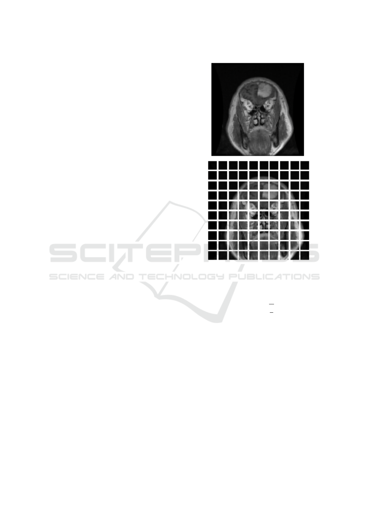
Figure 4: Splitting the image into patches.

(GELU) activation function. The GELU function is

computed as follows:

GELU (x) = 0.5x(1 + tanh(

(x + 0.044715x

)))

(6)

The main advantage of GELU is that it avoids van-

ishing gradients problem (Hendrycks and Gimpel,

2016). Most recent transformer network models, such

as BERT, or GPT-2 use this activation function (De-

vlin et al., 2019), (Radford and et al., 2019).

A block diagram showing the patch-based Vision

Transformer used in this work for tumor detectino and

classiﬁcation is shown in Fig. 5.

3.3 CNN Model

Most current image classiﬁcation tasks for medical

applications that involve deep learning rely on Convo-

lutional Neural Networks (Yamashita, 2017), (Koner

et al., 2020), (Dosovitskiy et al., 2021), with newer

ones only recently combining Transformers with

BIOIMAGING 2022 - 9th International Conference on Bioimaging

126

Figure 5: Vision Transformer (ViT) Architecture for detection/classiﬁcation of MRI brain tumors.

CNNs (Wang et al., 2021). In order to test the efﬁ-

ciency of ViT-alone compared to CNN-alone, we con-

struct a CNN network for our dataset and compare its

performance to that of ViT. Various CNN architec-

tures were tested, and after appropriate hyperparame-

ter optimization and experimentation we used the one

in Fig. 6 that led to the best results.

We compare our ViT results with those of our

CNN, and indirectly compare with the SoA CNN for

brain tumor classiﬁcation (Badza and Barjaktarovic,

2020). The CNN of (Badza and Barjaktarovic, 2020)

is not directly comparable with ours, as their CNN

involves more convolutional layers, the dataset split

they use is not known, and also carry out data aug-

mentation and k-fold validation. In our case, we only

implement our CNN to compare its “barebones” per-

formance with that of the ViT under the same condi-

tions (same dataset, same train/test split, no augmen-

tation). In this manner, we aim to objectively and

clearly showcase the effect of context and attention,

under the same experimental conditions.

4 EXPERIMENTS

In order to compare the efﬁciency of ViT-alone com-

pared to CNN-alone, we perform experiments for the

same train-test split on the data set, as explained

above. The idea is to train both models on 80% of

the data, while keeping the rest for validation/testing

purposes, so we used an 80/20 training/validation

split (Russell and Norvig, 2009). The accuracy of

the model is the percentage of correctly classiﬁed in-

stances. In order to compute it, we need to divide the

sum of the True Positive and True Negative terms by

the total number of testing instances. Another inter-

esting measure, for both binary and multi-class prob-

lem, is the confusion matrix. Indeed, the confusion

matrix shows, among all the possible classes, what

the predicted value is. The diagonal elements from

the matrix represent instances that have been correctly

classiﬁed.

4.1 Validation/Training

As a ﬁrst step in examining the performance of our

two models, we carried out validation experiments.

The validation set allows us to observe that the ViT

model is overﬁtting the data to a small degree, but

training loss remains very close to the validation loss,

or lower, making this a minimal effect. The CNN

slightly overﬁts the dataset (Fig. 8), which can be

attributed to the limited training data. Figs. 9, 10 with

the validation/training accuracies shows this is still

the case, but is not a signiﬁcant effect.

4.2 Classiﬁcation Performance

We examine the performance of both architectures

for the problem of tumor classiﬁcation for the four

classes of tumors Glioma, Meningioma, No Tumor,

Pituitary. The confusion matrix in Table 1 shows that

the ViT indeed accurately ﬁnds the classes with low

false positives. Table 2 shows it results in overall

accuracy of 96.5 %, and surpasses the CNN, which

achieves an accuracy of 89.78 %.

The current SoA on the same data achieves a 95.4

% classiﬁcation accuracy (Badza and Barjaktarovic,

2020) using a CNN-based approach. It should be

noted that we only indirectly compare our results to

theirs, as they do not make their code and all imple-

mentation details available. They also perform data

augmentation, increasing their CNN-based accuracy

to 96.4 %, which is very close to the accuracy we

achieved using ViTs. However, in the case of speciﬁc

applications like medical imaging, data augmentation

needs to be carefully applied, so as to not distort cru-

cial information in the medical images.

Vision Transformers for Brain Tumor Classiﬁcation

127

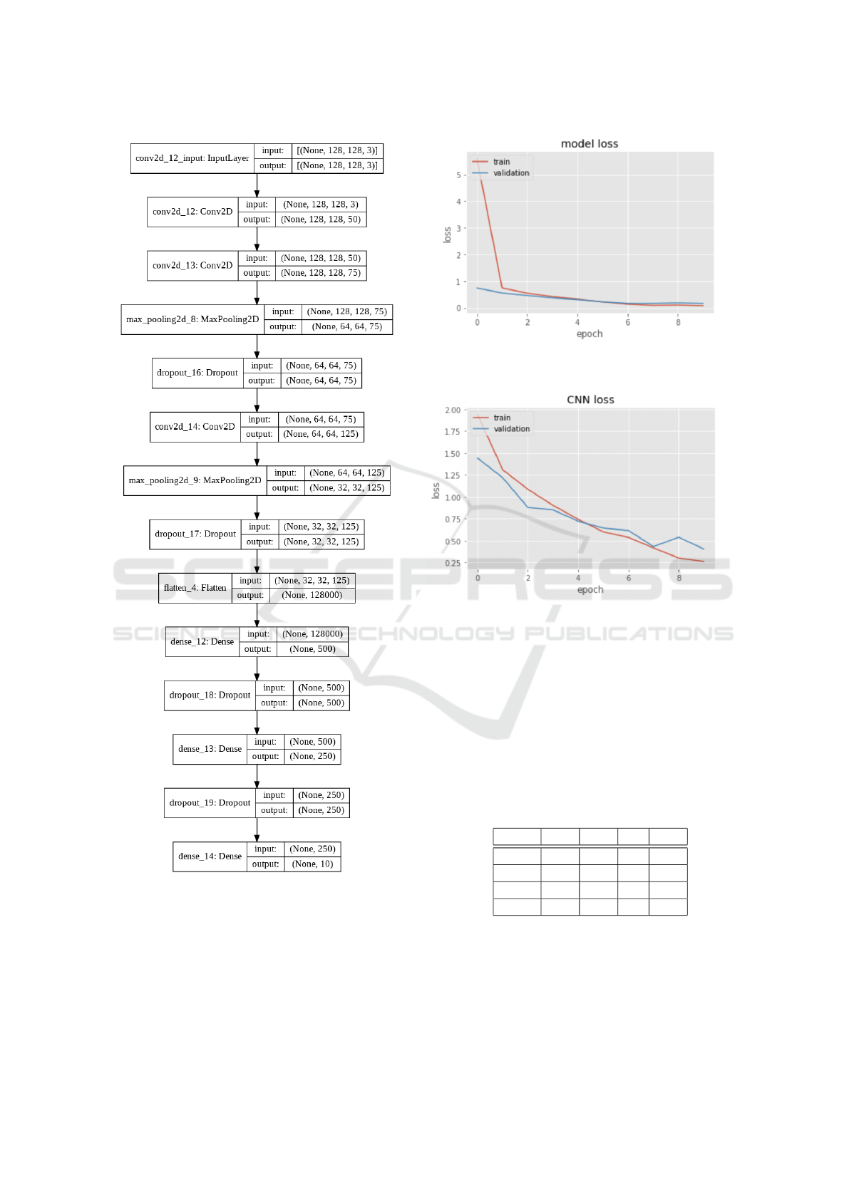
Figure 6: CNN model compared with Vision Transformers.

We carried out initial testing with data augmenta-

tion and observed that it can also worsen accuracy by

introducing unexpected distortions, and requires sig-

niﬁcantly more training time to achieve a decent ac-

curacy. This demonstrates that augmentation needs

to be implemented strategically to avoid such issues,

while it also entails a much higher computational

Figure 7: Model loss over time for the ViT for the validation

and training data.

Figure 8: Model loss over time for the CNN for the valida-

tion and training data.

cost, which increases even more when k-fold valida-

tion is involved. For these reasons, and in order to

avoid a computationally costly solution, we do not

proceed with data augmentation in these experiments,

and show we still achieve very high accuracies that

surpass our CNN under the exact same setup. Some

examples of correctly classiﬁed tumors by the ViT can

be seen in Fig. 11.

Table 1: Vision Transformer Confusion matrix for Classes:

1: Glioma, 2: Meningioma, 3: No Tumor, 4: Pituitary.

Class 1 2 3 4

1 139 5 3 0

2 2 172 1 0

3 1 0 76 0

4 0 0 0 178

4.3 Detection Performance (Binary

Case)

We also examine the performance of the CNN and

the ViT for the binary dataset containing samples of

BIOIMAGING 2022 - 9th International Conference on Bioimaging

128

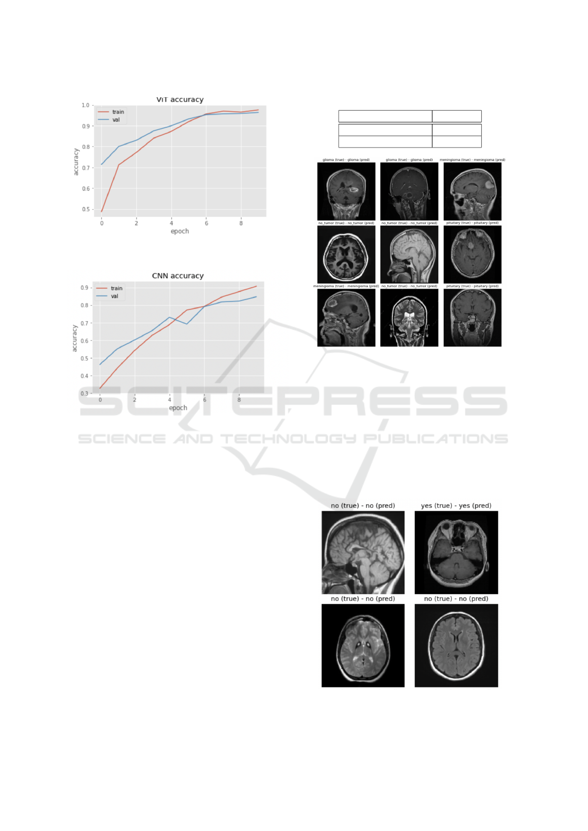
Figure 9: Model accuracy over time for the ViT for the val-

idation and training data.

Figure 10: Model accuracy over time for the CNN for the

validation and training data.

tumor vs no tumor. In this case, the confusion matrix

of Table 3 again shows the ViT correctly detects most

tumor/no tumor cases, with a few false alarms that

show it still does not overﬁt. Fig. 12 shows character-

istic samples that are correctly labeled as tumor/no tu-

mor by the ViT. In this simpler task, the ViT performs

very well, achieving an exceptionally high accuracy

of over 98 %, despite the dataset being unbalanced.

Although the binary classiﬁcation task can be con-

sidered simpler than that of four-class classiﬁcation

examined above, its large imbalance could introduce

errors to our data, such as missing the no tumor cases.

These good results can be attributed to the fact that at-

tention in ViT’s helps them focus on salient regions of

each image, achieving higher detection accuracy and

fewer false alarms introduced from other regions.

5 CONCLUSIONS

This research proposed applying recently introduced

Vision Transformer models to the challenging prob-

lems of brain tumor detection and classiﬁcation on a

Table 2: Final Accuracies for tumor classiﬁcation.

Classiﬁcation Model Accuracy

ViT 0.965

CNN 0.8978

Figure 11: ViT Model Prediction/Actual Label for tumor

classiﬁcation.

benchmark dataset. Vision Transformers were tested

as-is, i.e. without any convolutional layers, so as

to examine the effect of their spatial attention alone,

without the aid of translational invariance present in

CNNs. We trained the ViT from scratch on a bench-

marking dataset of relatively small size, that is quite

unbalanced, and avoided adding data augmentation

or cross-validation to examine its performance as-is,

and to reduce computational requirements. The ViT

model performed extremely well, also compared to

Figure 12: Binary case: ViT Model Prediction/Actual La-

bel.

Vision Transformers for Brain Tumor Classiﬁcation

129

Table 3: Vision Transformer Confusion matrix for the Bi-

nary Model (Tumor/No tumor).

Tumor Detection no tumor tumor

no tumor 99 7

tumor 2 497

our custom-built CNN trained under the same exact

conditions. Although the model did not train on a

huge amount of data, and used an unbalanced it still

managed to achieve 96.5 % classiﬁcation accuracy,

and over 98 % detection accuracy, which is impres-

sive. We compared to CNNs, which are used in the

SoA for such tasks, and demonstrated that the ViT

can still achieve better accuracy, despite lacking trans-

lational invariance. Some modiﬁcations could im-

prove the efﬁciency of the model, such as optimizing

the hyper-parameters. Adding another regularization

technique and appropriate data augmentation could

also ensure the model does not overﬁt the data. These

solutions entail another tradeoff, as they are likely to

signiﬁcantly increase training time to achieve good

accuracy. Finally, future work includes investigating

the use of recently introduced Convolutional Vision

Transformers (CvT), which attain higher results than

normal Vision Transformers.

REFERENCES

Badza, M. and Barjaktarovic, C. (2020). Classiﬁcation of

brain tumors from mri images using a convolutional

neural network. Applied Sciences.

Cho, K., van Merrienboer, B., G

ulc¸ehre, C¸ ., Bahdanau, D.,

Bougares, F., Schwenk, H., and Bengio, Y. (2014).

Learning phrase representations using RNN encoder-

decoder for statistical machine translation. In Mos-

chitti, A., Pang, B., and Daelemans, W., editors, Pro-

ceedings of the 2014 Conference on Empirical Meth-

ods in Natural Language Processing, EMNLP 2014,

October 25-29, 2014, Doha, Qatar, A meeting of

SIGDAT, a Special Interest Group of the ACL, pages

1724–1734. ACL.

Dai, Y., Y. Gao, Y., and Liu, F. (2021). Transmed: Trans-

formers advance multi-modal medical image classiﬁ-

cation. Diagnostics.

Devlin, J., Chang, M., Lee, K., and Toutanova, K. (2019).

BERT: pre-training of deep bidirectional transformers

for language understanding. In Burstein, J., Doran,

C., and Solorio, T., editors, Proceedings of the 2019

Conference of the North American Chapter of the As-

sociation for Computational Linguistics: Human Lan-

guage Technologies, NAACL-HLT 2019, Minneapolis,

MN, USA, June 2-7, 2019, Volume 1 (Long and Short

Papers), pages 4171–4186. Association for Computa-

tional Linguistics.

Dosovitskiy, A., Beyer, L., Kolesnikov, A., Weissenborn,

D., Zhai, X., Unterthiner, T., Dehghani, M., Minderer,

M., Heigold, G., Gelly, S., Uszkoreit, J., and Houlsby,

N. (2021). An image is worth 16x16 words: Trans-

formers for image recognition at scale. In Interna-

tional Conference on Learning Representations.

He, K., Zhang, X., Ren, S., and Sun, J. (2016). Deep resid-

ual learning for image recognition. In 2016 IEEE Con-

ference on Computer Vision and Pattern Recognition

(CVPR), pages 770–778.

Hendrycks, D. and Gimpel, K. (2016). Gaussian error linear

units (gelus). arXiv preprint arXiv:1606.08415.

Herholz, K. (2012). Brain tumors. PubMed.

Hossain, T., Tonmoy, F., Shishir, S., Ashraf, M., Nasim, A.,

and Shah, F. (2019). Brain tumor detection using con-

volutional neural network. In 2019 1st International

Conference on Advances in Science, Engineering and

Robotics Technology (ICASERT), pages 1–6.

ImageNet (2007). Imagenet benchmark (image classiﬁca-

tion), 2007. https://paperswithcode.com/sota/image-

classiﬁcation-on-imagenet.

Koner, R., Sinhamahapatra, P., and Tresp, V. (2020). Rela-

tion transformer network. CoRR, abs/2004.06193.

MRI Kaggle dataset (2020). Brain tu-

mor classiﬁcation (mri), 2020.

https://www.kaggle.com/sartajbhuvaji/brain-tumor-

classiﬁcation-mri.

Radford and et al. (2019). Language models are unsuper-

vised multitask learners. OpenAI.

Rehman, A., Naz, S., Razzak, I. M., Akram, F., and Im-

ran

a, M. (2019). A deep learning-based framework

for automatic brain tumors classiﬁcation using trans-

fer learning. Circuits, Systems, and Signal Processing.

Russell, S. J. and Norvig, P. (2009). Artiﬁcial Intelligence:

a modern approach. Pearson, 3 edition.

Scans (2021). Best scans to detect cancer.

https://www.envrad.com/best-scans-to-detect-cancer/.

Vaswani, A., Shazeer, N., Parmar, N., Uszkoreit, J., Jones,

L., Gomez, A., Kaiser, L., and Polosukhin, I. (2017).

Soft-gated warping-gan for pose-guided person image

synthesis. Advances in Neural Information Processing

Systems, pages 5998–6008.

Wang, Q., Li, B., Xiao, T., Zhu, J., Li, C., Wong, D., and

Chao, L. (2019). Learning deep transformer models

for machine translation. In 57th Annual Meeting of

the Association for Computational Linguistics (ACL)

2019, pages 1810–1822.

Wang, W., Chen, C., Ding, M., Li, J., Yu, H., and Zha, S.

(2021). Transbts: Multimodal brain tumor segmen-

tation using transformer. In 24th International Con-

ference on Medical Image Computing and Computer

Assisted Intervention (MICCAI 2021).

Warden (2017). How many images do

you need to train a neural network?

https://petewarden.com/2017/12/14/how-many-

images-do-you-need-to-train-a-neural-network/.

Yamashita, R. (2017). Convolutional neural networks: an

overview and application in radiology. Insights into

Imaging.

Zichao, Y. and et al. (2016). Hierarchical attention net-

works for document classiﬁcation. In Proceedings of

the 2016 Conference of the North American Chapter

of the Association for Computational Linguistics: Hu-

man Language Technologies, page 1480–1489.

BIOIMAGING 2022 - 9th International Conference on Bioimaging

130

REFERENCES

Badza, M. and Barjaktarovic, C. (2020). Classification of